A General Testing Problem in Linear Model

Posted on 2019-01-18 Edited on 2023-01-30 In Stat Model Word count in article: 3.4k Reading time ≈ 13 mins.

Model notation

The linear model notation we are using in this post is

\[ \text{E}(y)=X\beta \ \ ,\text{Var}(y)=\sigma^2I_n \] where $I_n$ is a $n \times n$ identity matrix and the distribution of $y$ is multivariate normal. $\hat{\beta}$ is the least square estimator of $\beta$ which minimized the sum of squares of the residuals.

A Testing Problem

The most general linear null hypothesis takes the form \[ H_0: \ \ C\beta=c \] where $C$ is a $q \times p$ matrix and $c$ is a $q \times 1$ vector of known constants. Without loss of generality, we can assume that $\text{rank}(C)=q$.

In this general framework it is rarely of interest to pose a one-sided alternative, and indeed there is no unique way to dene such a thing. The usual alternative is simply \[ H_1: \ \ C\beta \ne c \] i.e. that at least one of the $q$ linear functions does not take its hypothesized value.

Constructing a test

An obvious way to build a test is to consider the estimator $C \hat{\beta}$.

If the null hypothesis is true, we have \[ \text{E}(C \hat{\beta})=C\beta=c,\ \ \text{Var}(C \hat{\beta})=\sigma^2C(X^{T}X)^{-1}C^{T}. \] And so \[ C \hat{\beta} \sim N_q(c,\sigma^2C(X^{T}X)^{-1}C^{T}) \] If $H_0$ is true, we find that \[ (C \hat{\beta}-c)^T (C(X^{T}X)^{-1}C^{T})^{-1}(C \hat{\beta}-c)/\sigma^2 \sim \chi_q^2 \] Using the fact that if $X$ and $Y$ are independent random variables with $X \sim \chi_{v_1}^2$ and $Y \sim \chi_{v_2}^2$, then $\frac{X/v_1}{Y/V_2}$ has the $F_{v_1,v_2}$ distribution,

$$ \frac{(C \hat{\beta}-c)^T (C(X^{T}X)^{-1}C^{T})^{-1}(C \hat{\beta}-c)}{q \hat{\sigma}^2}\sim F_{q,n-p} \tag{*}\label{aa1} $$

We would expect this $(C \hat{\beta}-c)^T (C(X^{T}X)^{-1}C^{T})^{-1}(C \hat{\beta}-c)$ to be larger.

So for a $100(1-\alpha)$% significance test we will reject $H_0$ if the test statistic exceeds $F_{q,n-p,\alpha}$.

The upper $100(1-\alpha)$% point of the $F_{q,n-p}$ distribution.

This is a one-sided test, even though the original alternative was two-sided. It is one-sided because we are using sums of squares, so that any failure of the null hypothesis leads to a larger value of the test statistic.

It is one-sided because we are using sums of squares, so that any failure of the null hypothesis leads to a larger value of the test statistic.

Testing the effect of a subset of regressor variables

We now concentrate on the case where $C=(0\ \ I_q)$, where the $0$ is a $q \times (p-q)$ matrix of zeros, and $c=0$, a $q \times 1$ vector of zeros. Then if we define \[ \beta=\begin{pmatrix} \beta_1 \\\\ \beta_2 \end{pmatrix} \] such that $\beta_1$ is $(p-q)\times 1$ and $\beta_2$ is $q \times 1$ then $C \beta=\beta_2$ and $H_0$ just specifies that $\beta_2=0$.

The null hypothesis therefore asserts that the last $q$ regressor variables all have no effect on the dependent variable.

Notice that the order of elements in $\beta$ is arbitrary; we can always shuﬄe them if we simultaneously shuﬄe the same way the columns of $X$. Hence there is no restriction in assuming that the $q$ variables whose eﬀect we wish to test are the last $q$.

We can express the sums of squares, and corresponding tests, in an Analysis of Variance (or ANOVA) table.

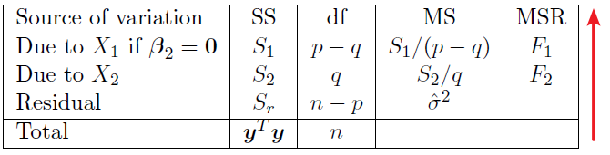
The two mean square ratios are $F_2=S_2/(q \hat{\sigma}^2)$ and $F_1=S_2/((p-q) \hat{\sigma}^2)$.

We have two tests that can be performed here:

Firstly, we reject the null hypothesis that $\beta_2=0$ at the $\alpha$ level of significance, if $F_2 \gt F_{q,n-p,\alpha}$.
Secondly, we uses $F_1$ and tests whether $\beta_1=0$ where we also assume that $\beta_2=0$ (i.e. we assume $\beta=0$ under the null hypothesis). We reject the null hypothesis that $\beta_1=0$, at the at the $\alpha$ level of significance if $F_1 \gt F_{p-q,n-p.\alpha}$.

注意以上两步不是完全正确的检验程序，因为假如如果我们不能拒绝$\beta_2=0$，那么这也不意味着这个假设是正确的。然而，这是公认的做法。

Adjusting for the constant term - the minimal model

When we say that the explanatory variables have no relationship with the dependent variable (i.e. they explain nothing), the implication would usually be that the expectation of $y$ is constant, no matter what the values of the explanatory variables. We would not usually think that the constant value would have to be zero.

Thus, linear models nearly always include a constant term, corresponding to a column of ones in X. This model is often called the minimal model (or null model).

当我们说解释变量与因变量没有关系时（即它们没有解释任何东西），其含义通常是：无论解释变量的值如何，y的期望值都是常数。我们通常不会认为这个常数必须是零。在上一节里我们假设了$c=0$以及$C=I$，这在一般实践中是很少见的。

The null hypothesis that the regressor variables have no eﬀect on y is usually that all the other elements of $\beta$ are zero. We can formulate this as in the ANOVA above.

We re-write the model as

\[ \beta=\begin{pmatrix}\beta_1 \\\\ \beta_2\end{pmatrix} \]

where $\beta_1=\beta_0$ is the first element of vector $\beta$ (即，$\beta_1$长度为1，是向量$\beta$的第一个元素), and the 1st column of $X$ is $X_1=1_n$. While, $\beta_2$ is remaining $p-1$ elements of $\beta$ corresponding to $p-1$ regressor variables in $X$.

$$ \overrightarrow{\beta}=(1,\overrightarrow{\beta_2})_{p \times 1} $$

and

$$ X=(X_1,X_{p-1})=\begin{bmatrix} 1 & x_{1,2} & \dots & x_{1,p} \\ 1 & x_{2,2} & \dots & x_{2,p}\\ \dots & \dots & \dots & \dots\\ 1 & x_{n,2} & \dots & x_{n,p} \end{bmatrix}_{n \times p} $$

The model with just $\beta_0$ in it is the simplest of all linear models, the case of a single normal sample with mean $\beta_0$ and variance $\sigma^2$.

In the present notation,

$$ \begin{matrix} S_1=y^TX_1(X_1^TX_1)^{-1}X_1^Ty=\frac{(\sum y)^2}{n}=n\bar{y}^2 \text{; (SS due to intercept)} \\\\ S_r=y^Ty-\hat{\beta}^TX^TX\hat{\beta} \text{; (SS due to residuals)} \end{matrix} $$

and this means

$$ S_2=y^Ty-S_1-S_r=\hat{\beta}^TX^TX\hat{\beta}-n\bar{y}^2 $$

After testing whether all but $\beta_0$ are zero we usually have no interest in testing whether $\beta_0=0$, so it is usual to omit the $S_1$ row of the ANOVA table.

So to test whether none of the explanatory variables has any eﬀect on $y$ (but allowing a constant term), we would use the same analysis of variance table as before with $q = p − 1$ and with the $S_1$ row omitted.

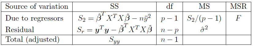
请注意，我们现在把总平方和看作是只用截距（$\mu$）对模型进行检验后的残差平方和 !

Now $S_{yy}=y^Ty-n\bar{y}^2$ and so $S_{yy}$ is indeed the sum of the SS column. The $\text{MSR is }F=\frac{S_2}{(p-1)\sigma^2}$, which we refer to tables of significance points of the $F_{p-1,n-p}$ distribution.

This approach extends to when we want to test for the eﬀect of a subset of the regressor variables, when we also have a constant term.

We would automatically adjust sums of squares to allow for the constant term. The resulting ANOVA table is

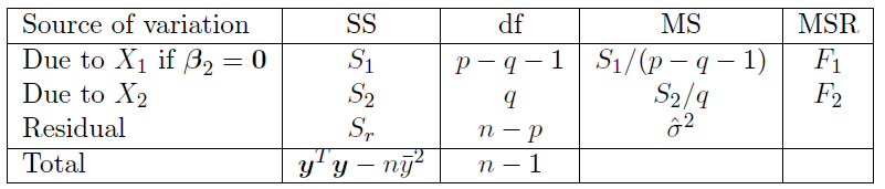
The details of the construction of this table are as follows.

We assume the number of regressor variables in $\beta_2$ is still $q$. It means that $\beta_1$ contains the constant term $\beta_0$ plus the remaining $p-q-1$ regressor variables.
The residual $\text{SS}$ and $\text{df}$ are unchanged, because they relate to the residuals after ﬁtting the constant plus all the other $p − 1$ regressor variables.
The $\text{SS}$ due to regressor variables $X_1$ is given by $S_1=y^TX_1(X_1^TX_1)^{-1}X_1^Ty-n\bar{y}^2=\hat{\beta_1}^TX_1^TX_1\hat{\beta_1}-n\bar{y}^2$
The $\text{SS}$ due to regressor variables $X_2$ is still $S_2=y^TM_2y=\hat{\beta_2}^TG_{qq}^{-1}\hat{\beta_2}$ but the alternative expression for it becomes $S_2=(\hat{\beta}^TX^TX\hat{\beta}-n\bar{y}^2)-S_1$, where in both expressions we correct for the constant term.

Here $M_2$ is related to the variance-covariance matrix of the residuals. $G_{qq}$ is the $q$-th diagonal element of $G=(X^TX)^{-1}$.

Testing nested models using F tests

Equation $\eqref{aa1}$ allows us to perform an important test in linear models.

This is where one of the models is nested within the other and we want to know whether adding the extra parameters increases the regression sums of squares enough to warrant the inclusion of the extra terms in the model.

For example we might have two models given by:

\[ y_i=\beta_0+\beta_1x_i; \\\\ y_i=\beta_0+\beta_1x_i+\beta_2x_i^2 \]

and we want to know whether $\beta_2 = 0$ so that the quadratic term does not increase the regression sums of squares enough to warrant inclusion in the model. These two models are nested because one model is the same as the other if we impose some constraints on the parameters ($\beta_2=0$ in the above example).

These tests are very important in model building as they allow us to determine which regressor variables we might need in our statistical model - they are a variable selection tool. These tests of nested models can be carried out using equation $\eqref{aa1}$ and this is equivalent to performing the following test (which is easier to implement).

Deﬁne the following:

$n$ is the number of observations
$p_f$ is the number of parameters in the full model
$p_r$ is the number of parameters in the reduced model
$RSS_f$ is the residual sums of squares in the full model
$RSS_r$ is the residual sums of squares in the reduced model

Then under the null hypothesis (that the coeﬃcients of the extra parameters are all zero)

\[ \frac{(RSS_r-RSS_f)/(p_f-p_r)}{(RSS_f)/(n-p_f)} \sim F_{p_f-p_r,n-p_f} \] These tests are performed in R using the anova command.

Example - The tractor data

The tractor data show the ages in years of 17 tractors and their maintenance costs (in pounds) per 6 months.

> tractor.data
   maint age
1    182 0.5
2    163 0.5
3    978 1.0
4    466 1.0
5    549 1.0
6    495 4.0
7    723 4.0
8    681 4.0
9    619 4.5
10  1049 4.5
11  1033 4.5
12   890 5.0
13  1522 5.0
14  1194 5.0
15   987 5.5
16   764 6.0
17  1373 6.0

We establish two models described above

1
2
3

tractor.linear.lm <- lm(maint~age, data=tractor.data)
tractor.quadratic <- lm(maint ~ age + I(age^2), data = tractor.data)
anova(tractor.linear.lm,tractor.quadratic)

ANOVA table

Analysis of Variance Table

Model 1: maint ~ age
Model 2: maint ~ age + I(age^2)
  Res.Df     RSS Df Sum of Sq     F Pr(>F)
1     15 1205407                          
2     14 1203176  1    2231.2 0.026 0.8743

Using the anova command with two nested linear models performs a test in which the null hypothesis is that the coeﬃcients of the ‘extra’ least squares parameters in the larger model are all zero, in this case \[ H_0:\beta_2=0 \text{ v.s. } H_1:\beta_2 \ne 0. \] In the R output above we can see that there is no to reject the null hypothesis $H_0:\beta_2=0$ and $p=0.8743$.

We can use the F-test for nested models directly giving \[ \frac{(RSS_r-RSS_f)/(p_f-p_r)}{(RSS_f)/(n-p_f)}=\frac{2231/(3-2)}{1203176/(17-3)}=0.026 \] as given in the R output.

1	anova(tractor.quadratic)

The output in the form of the ANOVA tables of quadratic model

Analysis of Variance Table

Response: maint
          Df  Sum Sq Mean Sq F value   Pr(>F)   
age        1 1099635 1099635  12.795 0.003034 **
I(age^2)   1    2231    2231   0.026 0.874295   
Residuals 14 1203176   85941                    
---
Signif. codes:  0 ‘***’ 0.001 ‘**’ 0.01 ‘*’ 0.05 ‘.’ 0.1 ‘ ’ 1

Rewriting it produces the easier to read ANOVA table below.

Source of Variation	SS	df	MS	MSR	P-val
($S_1$) Linear term if $\gamma=0$	1099635	1	1099635	12.8	0.003
($S_2$) Quadratic term	2231	1	2231	0.02	0.874
($S_r$) Residual	1203176	14	85941
Total	2305042	16

It is clear from the R output that as $p = 0.87$, there is not significant evidence to reject $H_0:\beta_2=0$, agreeing with the previous R output.

The other test in this table is whether $H_0:\beta_1=0$ given that $\beta_2=0$. Assuming that $\beta_2=0$, there is significant evidence $p=0.003$ to reject $H_0:\beta_1=0$. The linear term does significantly improve the fit.

Limitations of using sequential sums of squares as a variable selection tool

在进行变量选择时，我们必须从一组回归变量中选择那些我们希望在统计模型中出现的变量，因为它们有助于解释或说明我们数据中观察到的变化。

我们已经看到，ANOVA Table可以通过进行一系列的假设检验来作为比较嵌套模型（Nested Model）的一种方式。

然而，顺序平方和法（sequential sums of squares method）的一个问题是，它是一个顺序程序：

ANOVA Table中随后几行的平方和代表额外的平方和，假设前面的回归变量在模型中。因此，表中回归变量的顺序可能会影响我们的结论。

只有在回归变量不相关的情况下，ANOVA Table中的项的顺序才不重要。

一般来说，这只发生在设计好的实验中，即在精心选择的因子变量水平上进行观察。在没有这种特定设计的研究中，表格中项的顺序是很重要的。

Changing order of variables arbitrarily - quadratic model

> anova(lm(maint~age+I(age^2),data=tractor.data))
Analysis of Variance Table

Response: maint
          Df  Sum Sq Mean Sq F value   Pr(>F)   
age        1 1099635 1099635  12.795 0.003034 **
I(age^2)   1    2231    2231   0.026 0.874295   
Residuals 14 1203176   85941                    
---
Signif. codes:  0 ‘***’ 0.001 ‘**’ 0.01 ‘*’ 0.05 ‘.’ 0.1 ‘ ’ 1

Entering age^2 followed by age produces the following ANOVA table

> anova(lm(maint~I(age^2)+age,data=tractor.data))
Analysis of Variance Table

Response: maint
          Df  Sum Sq Mean Sq F value   Pr(>F)   
I(age^2)   1 1074330 1074330 12.5008 0.003294 **
age        1   27536   27536  0.3204 0.580323   
Residuals 14 1203176   85941                    
---
Signif. codes:  0 ‘***’ 0.001 ‘**’ 0.01 ‘*’ 0.05 ‘.’ 0.1 ‘ ’ 1

我们看到，两张表格中年龄的sums of squares ($\text{SS}$)是不一样的。

在第二种情况下，Age的$\text{SS}$是Age^2被剔除后的extra $\text{SS}$，而第一种情况下的$\text{SS}$是linear predictor中只有Age的$\text{SS}$。

如果Age和Age^2是不相关的，那么Age的$\text{SS}$在两个方差分析表中是一样的，假设检验的结论也是一样的；但显然Age和Age^2是相关的。

根据第一个ANOVA Table，我们将把Age纳入模型，但不包括Age^2。

在第二个ANOVA Table中，我们将包括Age^2，但不包括Age。对于两个高度相关的变量，使用基于sequential $\text{SS}$的ANOVA Table，第二个变量几乎都会被拒绝。

考虑下面这个例子：

Consider ftting the following model to the tractor data \[ y_i=\beta_0+\beta_1x_i+\beta_2x_i^2+\beta_3x_i^3+\beta_4x_i^4+\epsilon_i \] The ANOVA table is obtained as follows

> trac.quart.lm=lm(maint~age+I(age^2)+I(age^3)+I(age^4))
> anova(trac.quart.lm)
Analysis of Variance Table

Response: maint
          Df  Sum Sq Mean Sq F value   Pr(>F)   
age        1 1099635 1099635 17.2249 0.001346 **
I(age^2)   1    2231    2231  0.0350 0.854823   
I(age^3)   1   31195   31195  0.4886 0.497860   
I(age^4)   1  405902  405902  6.3581 0.026833 * 
Residuals 12  766079   63840                    
---
Signif. codes:  0 ‘***’ 0.001 ‘**’ 0.01 ‘*’ 0.05 ‘.’ 0.1 ‘ ’ 1

Suppose we want to test the null hypothesis that \[ H_0: \beta_3=\beta_4=0. \]

i.e.

\[ C=\begin{pmatrix} 0 & 0 & 0 & 1 & 0 \\ 0 & 0 & 0 & 0 & 1 \end{pmatrix}, \ \ c=\begin{pmatrix} 0 \\ 0 \end{pmatrix}. \]

Because of the order of the terms in the ANOVA table above, the sums of squares for Age^3 and Age^4 are the excess sums of squares ‘explained’ beyond that ‘explained’ by Age and Age^2.

Remember that for nested F-tests we are looking at whether the excess sums of squares (the diﬀerence in the sums of squares for the larger and smaller models) for the parameters in the null hypothesis is large enough for us to reject the null.

原假设中的参数的excess SS（“大”模型和“小”模型的SS的差异）是否大到足以让我们拒绝原假设

So the sums in the table are exactly the sums of squares that we want to do our F-test.

Our F test would take the form \[ F=\frac{(31195+405902)/2}{766079/12}=3.423, \] and $p=0.067$ using 1-pf(3.423,2,12) so not significant evidence to reject $H_0: \beta_3=\beta_4=0$.

Furthermore, we also want to test the null hypothesis that \[ H_0: \beta_1=\beta_3=0. \] So could we use the same ANOVA table to test the null hypothesis that $H_0: \beta_1=\beta_3=0$?

What we need is the excess sums of squares that Age and Age^3 explain beyond that explained by Age^2 and Age^4. Clearly the table doesn’t provide this information (the sums of squares for Age is the sums of squares explained without any other terms in the model). So can we do the test using an ANOVA table? Yes, but we need to change the order the terms enter R. We want Age^2 and Age^4 to come before Age and Age^3, which can be achieved using

> quart=lm(maint~I(age^2)+I(age^4)+age+I(age^3),data=tractor.data)
> anova(quart)
Analysis of Variance Table

Response: maint
          Df  Sum Sq Mean Sq F value   Pr(>F)   
I(age^2)   1 1074330 1074330 16.8285 0.001466 **
I(age^4)   1   18524   18524  0.2902 0.599968   
age        1   16373   16373  0.2565 0.621727   
I(age^3)   1  429736  429736  6.7315 0.023462 * 
Residuals 12  766079   63840                    
---
Signif. codes:  0 ‘***’ 0.001 ‘**’ 0.01 ‘*’ 0.05 ‘.’ 0.1 ‘ ’ 1

Our F test would take the form \[ F=\frac{(16373+429736)/2}{766079/12}=3.494, \] and $p=0.064$ using 1-pf(3.494,2,12) so not significant evidence to reject $H_0: \beta_1=\beta_3=0$.

Source of Variation	SS	df	MS	MSR	P-val
(\(S_1\)) Linear term if \(\gamma=0\)	1099635	1	1099635	12.8	0.003
(\(S_2\)) Quadratic term	2231	1	2231	0.02	0.874
(\(S_r\)) Residual	1203176	14	85941
Total	2305042	16