Background

The dataframe YouthSurvey in the YouthSurvey.RData workspace contains data on the tolerance of 16 youths to deviant behaviour. Each year, when participants were ages 11, 12, 13, 14, and 15, they filled out a nine-item instrument designed to assess their tolerance of deviant behavior.

Using a four-point scale (1 = very wrong, 2 = wrong, 3 = a little bit wrong, 4 = not wrong at all), they indicated whether it was wrong for someone their age to:

1. cheat on tests,
2. purposely destroy property of others,
3. use marijuana,
4. steal something worth less than five dollars,
5. hit or threaten someone without reason,
6. use alcohol,
7. break into a building or vehicle to steal,
8. sell hard drugs, or
9. steal something worth more than fifty dollars.

The data consists of 5 columns:

• id - an identification variable for each of the 16 youths included in the dataset
• Sex - an indicator variable taking the value ‘M’ if the respondent is male, and ‘F’ if female
• Exposure - this assesses the respondent’s self-reported exposure to deviant behavior at age 11. To obtain values of this predictor, participants estimated the proportion of their close friends who were involved in each of the same nine activities on a five-point scale (ranging from 0 = none, to 4 = all). The value of Exposure is the average of his or her nine responses
• Age - the age of the respondent
• Tolerance - the respondents average across the nine tolerance questions.

Data Set

Task

Use the data to investigate the tolerance level of youths as they progress through adolescence. Examples of the type of questions you may wish to consider, are whether there is a tendency for tolerance of deviant behaviour to either increase or decrease as they progress through ado- lescence, whether there is a significant difference between male and female youths (both in their average tolerance, and in the change in their tolerance through time), and whether previous exposure affects tolerance? There are of course many other questions you could investigate.

Predict the tolerance of a female youth chosen randomly from the same population, who reported an exposure of 1.6 to deviant behaviour. Finally, suppose that in addition, you are later told that this individual has a tolerance of 2.5 at age 15. Predict what her tolerance was when she was age 11.

It may be assumed that the respondents in this dataset were selected randomly from the population and that all respondents answered the questions independently of each other.

Solution

1
2
3
4
5
6

YouthSurvey$CenAge <- YouthSurvey$Age-11
YouthSurvey$id <- factor(YouthSurvey$id)
YouthSurvey$Sex <- factor(YouthSurvey$Sex)
YouthSurvey <- YouthSurvey[,-c(4)]
theme_set(theme_bw())
set.seed(12)

Exploratory Data Analysis

The data consists of 5 variables. The variable id is a factor with 16 levels, Sex is also a factor with 2 levels. The other 3 variables named Exposure, CenAge, Tolerance are all quantitative variables. Note that the values of CenAge equals to Age\(-11\), where Age is a variable in the original dataset. In this way, the intercept will make sense when CenAge\(=0\). In this report, we will treat Tolerance as the response variable.

1
2
3
4
5

fit1_1 <- lm(Tolerance~CenAge, data = YouthSurvey)
plot1_1 <- qplot(CenAge, Tolerance, aes(group = CenAge), geom = "boxplot",data=YouthSurvey)+
  theme(panel.grid.major = element_blank(),text = element_text(size=10))
plot1_2 <- plot1_1+geom_line(aes(x=CenAge,y=predict(fit1_1)),color="red")
grid.arrange(plot1_1,plot1_2,ncol=2)

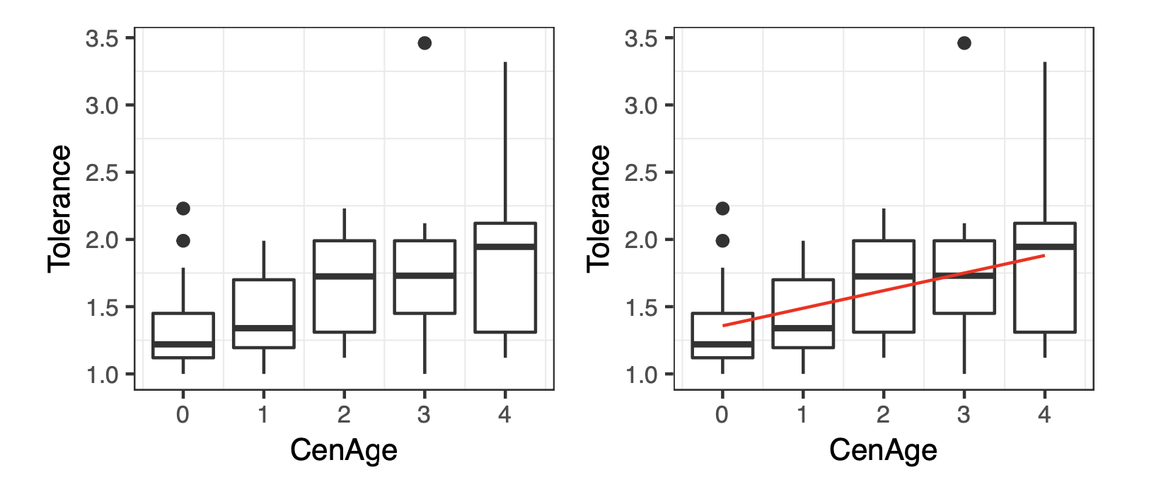
Figure 1: Tolerance versus CenAge for the YouthSurvey data

From the above Figure 1 we can see there is a tendency for tolerance of deviant behaviour to increase as age increases. The red trendline is fitted by a very simple linear regression model \(y_j=\beta_0+\beta_1\times\text{CenAge}_j+\epsilon_j,0\leqslant j \leqslant 4\), where \(\epsilon_j\sim N(0,\sigma^2)\), \(y_j\) is the observations of tolerance and \(\text{CenAge}_j\) is the value of explanatory variable \(\text{CenAge}_j\) when \(\text{CenAge}_j=j\):

1

fit1_1 <- lm(Tolerance~CenAge, data = YouthSurvey)

1
2
3
4
5
6
7

tempdf <- YouthSurvey
tempdf$pred <- fitted(fit1_1)
plot1_3 <- ggplot(data = tempdf)+
  geom_point(aes(x=CenAge, y=Tolerance))+
  geom_line(aes(x=CenAge,y=pred),color="red")+
  facet_wrap(~id,ncol=8)
plot1_3

Figure 2: Tolerance versus CenAge for 16 individuals, the red lines are the fitted lines based on model fit1_1

But this model is based on an assumption that the slope \(\beta_1\) and the intercept \(\beta_0\) are invariant for all individuals. Figure 2 shows facts that does not agree with the assumption: the parameters (i.e. slope and intercept) should vary from one individual to another. The model fit1_1 for each individual seems to underestimate or overestimate the individual tolerance of the 16 individuals. In fact, our study is based on 16 individuals selected randomly from the population. If we want to build global models for the whole population, it will be better to use mixed effect models in this case.

Fitting Mixed Effect Models for Explanation

Firstly, we want to explore whether there is a tendency for tolerance of deviant behaviour to either increase or decrease as they progress through adolescence. We assume that the initial tolerance (when CenAge\(=0\)) (i.e. the intercept) may depend on the individual (id). We can write a full model which contains the CenAge term and a reduced model respectively: \[ \begin{aligned} &\text{Full model: }y_{ij}=\beta_0+\beta_1 \times \text{CenAge}_{ij}+\eta_{i0}+\epsilon_{ij},\\ &\text{Reduced model: }y_{ij}=\beta_0+\eta_{i0}+\epsilon_{ij},\\ \end{aligned} \] where \(i\) is the index of each individual and \(i=1,2,\cdots,16\). The random effects \(\eta_{i0}\sim N(0,\sigma^2_b)\) and \(\epsilon_{ij}\sim N(0,\sigma^2)\) are independent of each other. We can use bootstrap hypothesis test to compare fixed effects structures and test \(H_0:\beta_1=0\).

1
2
3
4
5
6
7
8
9
10
11
12
13
14
15
16
17
18
19
20
21

# bootstrap function
fixef.comp.bootstrap <- function(repnum,reduced,full){
  N<-repnum
  l.test <-rep(0,N)
  fit_reduced <- eval(parse(text = paste("lmer(Tolerance~", reduced,
                                         ",data = YouthSurvey,REML = FALSE)",sep="")))
  fit_full <- eval(parse(text = paste("lmer(Tolerance~",full,
                                      ",data = YouthSurvey,REML = FALSE)",sep="")))
  l.obs <- -2*(logLik(fit_reduced)-logLik(fit_full))
  for(i in 1:N){
    y.new <- unlist(simulate(fit_reduced))
    fit_reduced_new <- eval(parse(text = paste("lmer(y.new~",reduced,
                                               ",data = YouthSurvey,REML = FALSE)",sep="")))
    fit_full_new <- eval(parse(text = paste("lmer(y.new~",full,
                                            ",data = YouthSurvey,REML = FALSE)",sep="")))
    l.test[i] <- -2*(logLik(fit_reduced_new)-logLik(fit_full_new))
  }
  cat("p-value: ",mean(l.test>=l.obs))
}
fixef.comp.bootstrap(repnum = 300,reduced = "1+(1|id)",
                     full = "CenAge+(1|id)")

p-value: 0

The output above suggests that the p-value for this test is smaller than 0.05, and it indicates that the tendency for tolerance of deviant behaviour as they progress through adolescence is statistically significant at the level of 0.05.

1
2

fit1_2 <- lmer(Tolerance~CenAge+(1|id),data = YouthSurvey)
fixef(fit1_2)

(Intercept) CenAge

1.3577500 0.1308125

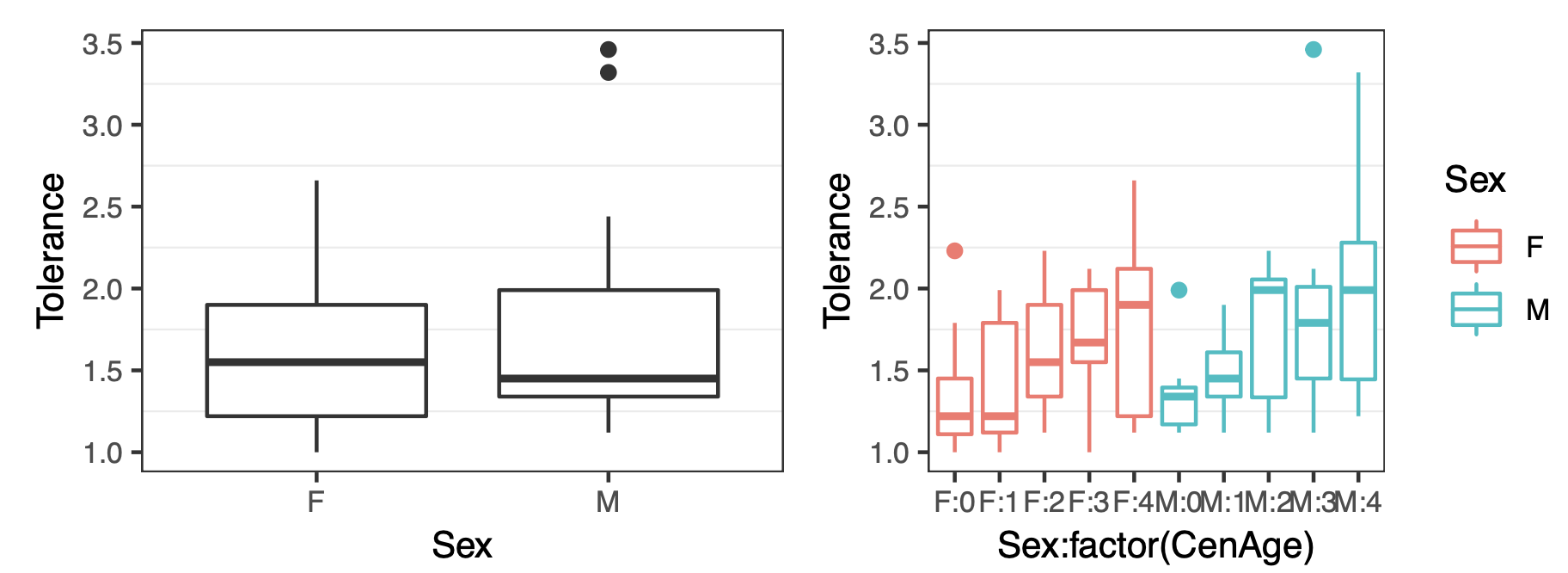
Figure 3: Tolerance versus Sex and Tolerance versus Sex in different age

From the output above, we can infer that the their tolerance will increase with an increase in their age. In Figure 3, it will be better to give some variation to the tendency for each individual. Therefore, we can update the full model to: \[ y_{ij}=\beta_0+\beta_1 \times \text{CenAge}_{ij}+\eta_{i0}+\eta_{i1}\times\text{CenAge}_{ij}+\epsilon_{ij}, \] where \(\eta_{i0}\sim N(0,\sigma^2_b)\),\(\eta_{i1}\sim N(0,\sigma^2_a)\), and \(\epsilon_{ij}\sim N(0,\sigma^2)\) with all the random effects independent of each other. Here we set uncorrelated random intercept and random slope within each individual. We are now trying to explore whether there is a significant difference between male and female youths in their average tolerance. Similarly, we can fit two models with the same random effect structure and use bootstrap hypothesis test to test the effect of a specific term in the fixed effect structure.

\[ \begin{aligned} &\text{Full model: }y_{ij}=\beta_0+\beta_{0M}\times\mathbb{I}_{\text{Sex}_i=M}+\beta_1 \times \text{CenAge}_{ij}+\eta_{i0}+\eta_{i1}\times\text{CenAge}_{ij}+\epsilon_{ij},\\ &\text{Reduced model: }y_{ij}=\beta_0+\beta_1 \times \text{CenAge}_{ij}+\eta_{i0}+\eta_{i1}\times\text{CenAge}_{ij}+\epsilon_{ij},\\ \end{aligned} \] where \(\mathbb{I}\) is the indicator function, and \(M\) is the abbreviation of male. We will use the code below to test \(H_0:\beta_{0M}=0\):

1
2

fixef.comp.bootstrap(repnum = 300,reduced = "1+CenAge+(CenAge-1|id)+(1|id)",
                     full = "CenAge+Sex+(CenAge-1|id)+(1|id)")

p-value: 0.7733333

The p-value above indicate that the difference between male and female youths in their average tolerance is not statistically significant at the level of 0.05. As for the question whether there is a significant difference between male and female youths in the change in their tolerance through time, we would like to compare these two models:

\[ \begin{aligned} &\text{Full model: }y_{ij}=\beta_0+\beta_{0M}\times\mathbb{I}_{\text{Sex}_i=M}+\beta_{1M}\times\mathbb{I}_{\text{Sex}_i=M}\times\text{CenAge}_{ij}+\beta_1 \times \text{CenAge}_{ij}+\eta_{i0}+\eta_{i1}\times\text{CenAge}_{ij}+\epsilon_{ij},\\ &\text{Reduced model: }y_{ij}=\beta_0+\beta_{0M}\times\mathbb{I}_{\text{Sex}_i=M}+\beta_1 \times \text{CenAge}_{ij}+\eta_{i0}+\eta_{i1}\times\text{CenAge}_{ij}+\epsilon_{ij},\\ \end{aligned} \] We will use the code below to test \(H_0:\beta_{1M}=0\). Note that \(\beta_{1M}\) is the deviation of the tendency for tolerance of deviant behaviour as they progress through adolescence for boys and girls.

1
2

fixef.comp.bootstrap(repnum = 300,reduced = "Sex+CenAge+(CenAge-1|id)+(1|id)",
                     full = "CenAge*Sex+(CenAge-1|id)+(1|id)")

p-value: 0.4833333

The p-value above indicate that the difference between male and female youths in the change in their tolerance through time is not statistically significant at the level of 0.05. From Figure 3, we can easily and clearly find out there is no visual difference between male and female youths both in their average tolerance and in the change in their tolerance through time.

1
2
3
4
5
6
7

plot2_1 <- qplot(Sex, Tolerance, geom = "boxplot",data=YouthSurvey)+
  theme_bw()+
  theme(panel.grid.major = element_blank(),text = element_text(size=10))
plot3_1 <- qplot(Sex:factor(CenAge), Tolerance, geom = "boxplot",data=YouthSurvey, col = Sex)+
  theme_bw()+
  theme(panel.grid.major = element_blank(),text = element_text(size=10))
grid.arrange(plot2_1,plot3_1,ncol=2)

As for the question whether previous exposure affects tolerance, we can use two models without the interaction term CenAge*Sex to make comparison. The null hypothesis will be \(H_0:\beta_{2}=0\).

\[ \begin{aligned} &\text{Full model: }y_{ij}=\beta_0+\beta_{0M}\times\mathbb{I}_{\text{Sex}_i=M}+\beta_1 \times \text{CenAge}_{ij}+\beta_2 \times \text{Exposure}_{i}+\eta_{i0}+\eta_{i1}\times\text{CenAge}_{ij}+\epsilon_{ij},\\ &\text{Reduced model: }y_{ij}=\beta_0+\beta_{0M}\times\mathbb{I}_{\text{Sex}_i=M}+\beta_1 \times \text{CenAge}_{ij}+\eta_{i0}+\eta_{i1}\times\text{CenAge}_{ij}+\epsilon_{ij},\\ \end{aligned} \]

1
2

fixef.comp.bootstrap(repnum = 500,reduced = "1+Sex+CenAge+(CenAge-1|id)+(1|id)",
                     full = "CenAge+Sex+Exposure+(CenAge-1|id)+(1|id)")

p-value: 0.046

The p-value given above is close to our chosen alpha (\(\alpha=0.05\)), there is evidence to reject the null hypothesis. We can say previous exposure may affect tolerance to some extent. Now we would like to use AIC to compare the following models that may be used for prediction. The reduced model is the model without the Sex term that is not statistically significant.

1
2
3
4

Full.to.pred <- lmer(Tolerance~CenAge+Sex+Exposure+(1|id)+(CenAge-1|id), data = YouthSurvey,REML = F)
Full.to.pred.reduced <- lmer(Tolerance~1+CenAge+Exposure+(1|id)+(CenAge-1|id), data = YouthSurvey, 
                             REML = F)
kable(data.frame(anova(Full.to.pred,Full.to.pred.reduced)))

According to Shmueli(2010), the AIC is better suited to model selection for prediction as it is asymptotically equivalent to leave-one-out cross-validation in regression, or one-step-cross-validation in time series. On the other hand, it might be argued that the BIC is better suited to model selection for explanation, as it is consistent. BIC penalizes model complexity more heavily. As for the p-values, they are associated with explanation, not prediction. It makes little sense to use p-values to determine the variables in a model that is being used for prediction. From the output above, we prefer to use model Full.to.pred.reduced to make prediction.

Fitting Mixed Effect Models for Prediction

The model we want to use to make prediction is: \[ y_{ij}=\beta_0+\beta_1 \times \text{CenAge}_{ij}+\beta_2 \times \text{Exposure}_{i}+\eta_{i0}+\eta_{i1}\times\text{CenAge}_{ij}+\epsilon_{ij}, \] where \(\eta_{i0}\sim N(0,\sigma^2_b)\),\(\eta_{i1}\sim N(0,\sigma^2_a)\), and \(\epsilon_{ij}\sim N(0,\sigma^2)\) with all the random effects independent of each other. Firstly, we would like to check these assumptions:

(1)The random effects \(\eta_{i0}\) are i.i.d. \(N(0,\sigma^2_b)\);

(2)The random effects \(\eta_{i1}\) are i.i.d. \(N(0,\sigma^2_a)\);

(3)The residual errors \(\epsilon_{ij}\) are i.i.d. \(N(0,\sigma^2)\);

(4)The fixed effects \(\beta_0\), \(\beta_1\), \(\beta_2\) adequately represent the mean response.

1
2
3

# We rename the Full.to.pred.reduced as Full.to.pred
Full.to.pred <- lmer(Tolerance~CenAge+Exposure+(1|id)+(CenAge-1|id),data = YouthSurvey)
summary(Full.to.pred)

1
2
3
4
5
6
7
8
9
10
11
12
13
14
15
16
17
18
19
20
21
22
23
24
25
26
27

> Linear mixed model fit by REML ['lmerMod']
> Formula: Tolerance ~ CenAge + Exposure + (1 | id) + (CenAge - 1 | id)
>    Data: YouthSurvey
>
> REML criterion at convergence: 70.8
>
> Scaled residuals:
>     Min      1Q  Median      3Q     Max
> -1.9389 -0.5651 -0.1463  0.3957  2.5044
>
> Random effects:
>  Groups      Name            Variance   Std.Dev.
>  id                (Intercept) 0.02285  0.1512
>  id.1             CenAge      0.01529  0.1236
>  Residual                        0.08094  0.2845
> Number of obs: 80, groups:  id, 16
>
Fixed effects:
         Estimate Std. Error t value
(Intercept)  0.91580    0.23912   3.830
CenAge       0.13081    0.03823   3.422
> Exposure     0.37100    0.19274   1.925
>    
> Correlation of Fixed Effects:
>       (Intr) CenAge
> CenAge   -0.111
>Exposure -0.960  0.000

1
2
3
4
5
6
7
8
9
10
11
12
13

par(mfrow=c(2,3))
qqnorm(ranef(Full.to.pred)$id[["(Intercept)"]],main = "QQplot for Assumption (1)")
abline(0,0.1522,col="red")
qqnorm(ranef(Full.to.pred)$id[["CenAge"]],main = "QQplot for Assumption (2)")
abline(0,0.1236,col="red")
qqnorm(resid(Full.to.pred),main = "QQplot for Assumption (3)(4)")
abline(0,0.2845,col="red")
plot(fitted(Full.to.pred),resid(Full.to.pred))
fix.fitted <- Full.to.pred@pp$X %*% fixef(Full.to.pred)
resid.random <- YouthSurvey$Tolerance - fix.fitted
plot(fix.fitted,resid.random)
plot(fitted(Full.to.pred),YouthSurvey$Tolerance)
abline(0,1,col="red")

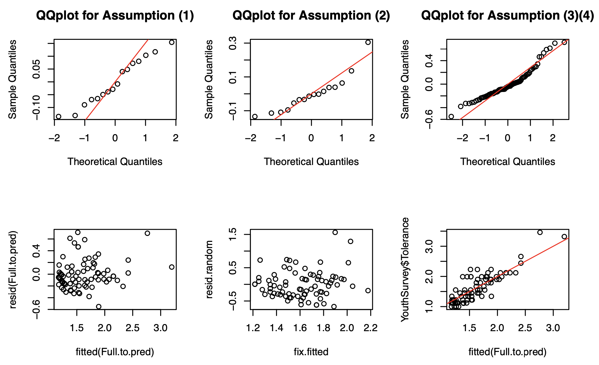
Figure 4: The plots on first row are for checking assumptions, and those plots on second row from left to right are subject-level residuals versus fitted values, population-level residuals versus fitted values, real tolerance versus fitted tolerance

Figure 5: Tolerance versus CenAge for 16 individuals, the red lines are the fitted lines based on model Full.to.pred

Overall, Figure 4 shows that the model is quite convicing. From Figure 5, it is obvious that the mixed effect model Full.to.pred make better prediction for each individual compared to model fit1_1.

1
2
3
4
5
6

q1.df <- YouthSurvey
q1.df$Full_pred <- fitted(Full.to.pred)
ggplot(data = q1.df)+
  geom_point(aes(x=CenAge, y=Tolerance))+
  geom_line(aes(x=CenAge,y=Full_pred),color="red")+
  facet_wrap(~id,ncol=8)

We want to predict the tolerance of a female youth chosen randomly from the same population who reported an exposure of 1.6 to deviant behaviour. Since the expectation of of \(y_{ij}\) could be written as:

\[ \begin{aligned} E(y_{ij})&=E(\beta_0+\beta_1 \times \text{CenAge}_{ij}+\beta_2 \times \text{Exposure}_{i}+\eta_{i0}+\eta_{i1}\times\text{CenAge}_{ij}+\epsilon_{ij})\\ &=\beta_0+\beta_1 \times \text{CenAge}_{ij}+\beta_2 \times \text{Exposure}_{i} \end{aligned}, \]

we can use the known coefficients of fixed effects to calculate the predicted tolerance of this female and 95% confidence interval of each predicted value. Note that we should firstly use bootstrap to calculate the 95% confidence interval for each coefficient of fixed effects.

1
2
3
4
5
6
7
8
9
10
11
12
13
14
15
16

x.new <- matrix(c(rep(1,5),c(0,1,2,3,4),rep(1.6,5)),nrow = 5)
fix.coef <- matrix(unlist(fixef(Full.to.pred)),nrow=3,
                   dimnames = list(c(),"Predicted Tolerance"))
pred_5_1 <- x.new %*% fix.coef
rownames(pred_5_1) <- c("Age 11","Age 12","Age 13","Age 14","Age 15")
N <- 1000
fixed.effect <- matrix(0,N,3)
for (i in 1:N){
  new.y <- unlist(simulate(Full.to.pred))
  new.full.to.pred <- lmer(new.y~CenAge+Exposure+(1|id)+(CenAge-1|id),
                           data = YouthSurvey)
  fixed.effect[i,]<-fixef(new.full.to.pred)
}
fixef.CI <- matrix(apply(fixed.effect,2,quantile,probs=c(0.025,0.975)),nrow = 2,
                   dimnames = list(c("2.5%","97.5%"),c("Intercept","CenAge","Exposure")))
cbind(pred_5_1,x.new %*% t(fixef.CI))

  Predicted Tolerance      2.5%    97.5%
  

Age 11 1.509397 0.4648572 2.554590

Age 12 1.640209 0.5196731 2.758646

Age 13 1.771022 0.5744890 2.962703

Age 14 1.901834 0.6293049 3.166759

Age 15 2.032647 0.6841208 3.370816

In addition, we are told that this girl has a tolerance of 2.5 at age 15. We need to use this information to calculate the random effects for her. Note that we use CenAge\(=4\) and CenAge\(=0\) to denote Age\(=15\) and Age\(=11\). For this female, we have

\[ \bigl(\begin{smallmatrix} Y_{new,15}\\ Y_{new,11} \end{smallmatrix}\bigr)\sim N \left ( \bigl(\begin{smallmatrix} m_{new,15}\\ m_{new,11} \end{smallmatrix}\bigr),\bigl(\begin{smallmatrix} V_{11} & V_{12}\\ V_{21} & V_{22} \end{smallmatrix}\bigr) \right ). \]

There for we can derive that \(E(Y_{new,CenAge=0}\mid Y_{new,CenAge=4})=m_{new,CenAge=0}+V_{21}V^{-1}_{11}\left ( Y_{new,CenAge=4}-m_{new,CenAge=4} \right )\), where \(m_{new,CenAge=0}\) is the fixed effect that we can use the method we just used above to calculate.

Since for a mixed effect model written by matrix notation \(\mathbf{Y}=\mathbf{X}\mathbf{\beta}+\mathbf{Z}\mathbf{b}+\mathbf{\epsilon}\), \(V_{21}V^{-1}_{11}\left ( Y_{new,CenAge=4}-m_{new,CenAge=4} \right )\) is the same thing as the estimated BLUP which is \(\widehat{\text{BLUP}}(\mathbf{b})=\widehat{C}_{b,Y}\widehat{V}^{-1}_{Y}(\mathbf{Y}-\mathbf{X}\widehat{\mathbf{\beta}})\). For each term, \(\widehat{C}_{b,Y}=(\mathbf{Z}\widehat{Var(\mathbf{b})})'\), \((\mathbf{Z}\widehat{(Var(\mathbf{b}))}\mathbf{Z}'+\widehat{\sigma}^2I)^{-1}\).

In this case, from the summary of model Full.to.pred, \(\mathbf{Y}=2.5\), \(\mathbf{X}=(1,4,1.6)\), \(\widehat{\mathbf{\beta}}=(0.91580,0.13081,0.37100)'\), \(\mathbf{Z}=(1,4)\), \(\widehat{\sigma}^2=0.08094\), \(I=1\), and \(\widehat{Var(\mathbf{b})}=\begin{pmatrix}0.02285 & 0\\ 0 & 0.01529\end{pmatrix}\). Put all of these values into the formula \(\widehat{\text{BLUP}}(\mathbf{b})=\widehat{C}_{b,Y}\widehat{V}^{-1}_{Y}(\mathbf{Y}-\mathbf{X}\widehat{\mathbf{\beta}})\) then we can get the random effects for this female. All calculations are done by the following code:

1
2
3
4
5
6
7
8
9
10
11
12
13
14
15

# Var(b)
var.b <- diag(c(0.02285,0.01529))
# Z
Z <- matrix(c(1,4),nrow = 1)
# Calculate random effects for this female
ranef5_2 <- (t(var.b) %*% t(Z))%*%
  solve(Z %*% var.b %*% t(Z)+0.08094*1)%*%
              (2.5-x.new[5,]%*%diag(3)%*%fix.coef)
cat("The random effects is: ", ranef5_2, "\n")
# Calculate fixed effects for this female at CenAge 0
x.5_2 <- matrix(c(1,0,1.6),nrow = 1)
z.5_2 <- matrix(c(1,0),nrow = 1)
# Calculate E(y_new_11|y_new_15)
cat("The predicted tolerance for the female when she was at age 11: ",
    (x.5_2%*%fix.coef+z.5_2%*%ranef5_2)[1,1])

The random effects is: 0.03064899 0.08203467

The predicted tolerance for the female when she was at age 11: 1.540046

Reference

Shmueli, Galit. To Explain or to Predict?. Statist. Sci. 25 (2010), no. 3, 289--310. doi:10.1214/10-STS330.