PoC Sample for ORR (Simulation)
This work tries to replicate the results from the following papers or slides.
- An Evidence Based Approach for Phase II Proof-of-Concept Trial
- Bayesian Design of Proof-of-Concept Trials
- Beyond p-values: A phase II dual-criterion design with statistical significance and clinical relevance
Key concepts
Minimally informative
A lot of the skepticism about Bayesian models comes from the assumptions that go into choosing a prior. Ideally the prior comes from real prior information, which we try to build in to the model in an intelligent and disciplined manner. If though, there is no prior information, or we are not confident in what is known, we can specify a prior that is not too influential. Termed non-informative or minimally informative, these priors will not weight or update the MLE from the data very much or at all, and the Bayesian results will be identical to the classical results.
In the 1950’s Sir Harold Jeffreys described an approach or general scheme for selecting minimally informative priors that now bears his name. It involves setting the prior equal to the square root of the expected Fisher information.
Find the minimum sample size n
Algorithm
Grid search:
- let r=1, increase n from, say 20, to 30; if violate CLINICAL RELAVANCE, stop; Record current n as n1;
- let r=r+1=2, increase n from n1 to 30 (assume n1<30), repeat the step above until violating CLINICAL RELAVANCE;
- repeat above steps;
- if all combination (r,n) (n>n_min) meet both STATISTICAL SIGNIFICANCE and CLINICAL RELAVANCE, then n_min is the minimum sample size.
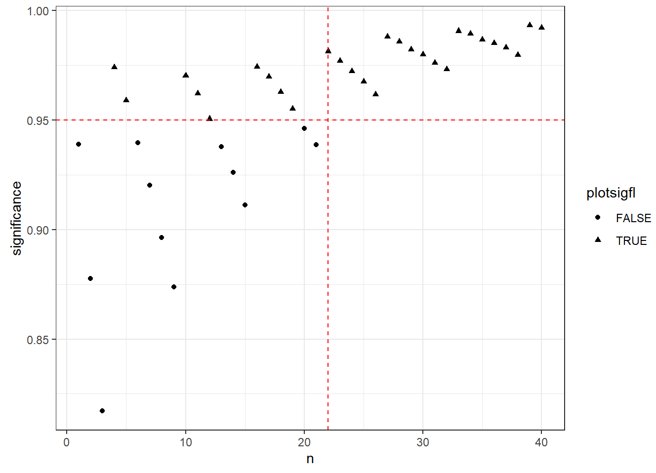
Note that we can find such n_min via visualization
1 | library(dplyr) |
Simulation
Scenario 1 (Dual Criterion)
- \(\alpha=0.05\), DV=0.175, n=25;
- True ORR (%) = 7.5, 12.5, 17.5, 22.5, 27.5
- GO: r>=5
- NOGO: r<5
Why for n=25, the minimum number of responders for a GO is 5?
We can see that if the #responders < 5, both criteria are missed and NO-GO decision will be made.1
2
3
4
5
6
7
8
9
10
11
12
13
14
15
16
17
18
19
20
21
22
23
24alpha <- 0.05
dv <- 0.175
nv <- 0.075
ssn <- 25
beta_a=0.0811
beta_b=1
r_vec <- 1:10
result1 <- matrix(NA,nrow = 3,ncol=10)
result1[1,] <- r_vec
# statistical significance and posterior median
for (r in r_vec){
rand <- rbeta(10000,beta_a+r,beta_b+ssn-r)
sig <- mean(rand>=nv)
med <- median(rand)
result1[2,r] <- sig
result1[3,r] <- med
}
df1 <- data.frame(result1)
row.names(df1) <- c("r","statsig","postmedian")
df1 %>%
kbl(caption = "minimum responders, n=25") %>%
kable_classic(full_width = F)
Simulate power: Scen1
From the above, we see that when n=25:
- r<5: both criteria will be violated, a NO-GO will be made;
- r>=5: both criteria will be achieved, a GO will be made;
so there is no space for a INCONCLUSIVE decision.1
2
3
4
5
6
7
8
9
10
11
12
13
14
15
16
17
18
19
20
21
22
23
24
25
26
27
28
29
30
31
32
33
34
35
36
37
38
39
40
41
42
43
44
45
46
47
48
49# function to simulate
sim_binom <- function(orr){
# parameters
alpha <- 0.05
dv <- 0.175
ssn <- 25
# responder for GO/NOGO
r_go <- 5
r_nogo <- 5
# simulate responders from binomial distribution
r <- sum(rbinom(ssn,1,orr))
goprob <- ifelse(r>=r_go,TRUE,FALSE)
nogoprob <- ifelse(r<r_nogo,TRUE,FALSE)
return(c(goprob,nogoprob))
}
# replicate trial to get GO/NO-GO possibilities.
rep_trial=5000
# set seed
set.seed(12)
# orr list
trueORR <- c(7.5, 12.5, 17.5, 22.5, 27.5)*0.01
# sim
resulttotal1 <- data.frame(matrix(0,nrow=5,ncol=4))
colnames(resulttotal1) <- c("true_orr","go","no-go","inconclusive")
i <- 1
for (o in trueORR) {
# simulate 1000 datasets over true ORR vector
df11 <- data.frame(t(replicate(rep_trial, sim_binom(orr = o))))
# Get mean of cols
df12 <- df11 %>% summarise(
orr = o,
successrate = mean(X1),
failrate = mean(X2),
incon = 1 - successrate - failrate
)
resulttotal1[i,] <- df12[1,]
i <- i+1
}
resulttotal1 %>%
kbl(caption = "operating characteristics, n=25") %>%
kable_classic(full_width = F)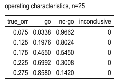
Scenario 2 (Dual Criterion)
- \(\alpha=0.05\), DV=0.175, n=36;
- True ORR (%) = 7.5, 12.5, 17.5, 22.5, 27.5
- GO: r>=7
- NOGO: r<=5
Why for n=36, the minimum number of responders for a GO is 7?
We can see that
- if the #responders > 7, both criteria are achieved and GO decision will be made.
- if the #responders <= 5, both criteria are missed and NO-GO decision will be made.
- if the #responders = 6, one criterion will be missed and INCONCLUSION will be made.
1 | alpha <- 0.05 |

Simulate power: Scen2
power simulation:1
2
3
4
5
6
7
8
9
10
11
12
13
14
15
16
17
18
19
20
21
22
23
24
25
26
27
28
29
30
31
32
33
34
35
36
37
38
39
40
41
42
43
44
45
46
47
48
49# function to simulate
sim_binom <- function(orr){
# parameters
alpha <- 0.05
dv <- 0.175
ssn <- 36
# responder for GO/NOGO
r_go <- 7
r_nogo <- 5
# simulate responders from binomial distribution
r <- sum(rbinom(ssn,1,orr))
goprob <- ifelse(r>=r_go,TRUE,FALSE)
nogoprob <- ifelse(r<=r_nogo,TRUE,FALSE)
return(c(goprob,nogoprob))
}
# replicate trial to get GO/NO-GO possibilities.
rep_trial=5000
# set seed
set.seed(12)
# orr list
trueORR <- c(7.5, 12.5, 17.5, 22.5, 27.5)*0.01
# sim
resulttotal1 <- data.frame(matrix(0,nrow=5,ncol=4))
colnames(resulttotal1) <- c("true_orr","go","no-go","inconclusive")
i <- 1
for (o in trueORR) {
# simulate 1000 datasets over true ORR vector
df11 <- data.frame(t(replicate(rep_trial, sim_binom(orr = o))))
# Get mean of cols
df12 <- df11 %>% summarise(
orr = o,
successrate = mean(X1),
failrate = mean(X2),
incon = 1 - successrate - failrate
)
resulttotal1[i,] <- df12[1,]
i <- i+1
}
resulttotal1 %>%
kbl(caption = "operating characteristics, n=36") %>%
kable_classic(full_width = F)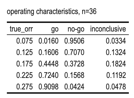
Scenario 3 (Standard 3 outcome design)
- \(\alpha=0.05\), n=27;
- True ORR (%) = 7.5, 12.5, 17.5, 22.5, 27.5
- GO: r>=5
- NOGO: r<=3
- INCONCLUSIVE: r=4
power simulation:1
2
3
4
5
6
7
8
9
10
11
12
13
14
15
16
17
18
19
20
21
22
23
24
25
26
27
28
29
30
31
32
33
34
35
36
37
38
39
40
41
42
43
44
45
46
47# function to simulate
sim_binom <- function(orr){
# parameters
ssn <- 27
# responder for GO/NOGO
r_go <- 5
r_nogo <- 3
# simulate responders from binomial distribution
r <- sum(rbinom(ssn,1,orr))
goprob <- ifelse(r>=r_go,TRUE,FALSE)
nogoprob <- ifelse(r<=r_nogo,TRUE,FALSE)
return(c(goprob,nogoprob))
}
# replicate trial to get GO/NO-GO possibilities.
rep_trial=5000
# set seed
set.seed(12)
# orr list
trueORR <- c(7.5, 12.5, 17.5, 22.5, 27.5)*0.01
# sim
resulttotal1 <- data.frame(matrix(0,nrow=5,ncol=4))
colnames(resulttotal1) <- c("true_orr","go","no-go","inconclusive")
i <- 1
for (o in trueORR) {
# simulate 1000 datasets over true ORR vector
df11 <- data.frame(t(replicate(rep_trial, sim_binom(orr = o))))
# Get mean of cols
df12 <- df11 %>% summarise(
orr = o,
successrate = mean(X1),
failrate = mean(X2),
incon = 1 - successrate - failrate
)
resulttotal1[i,] <- df12[1,]
i <- i+1
}
resulttotal1 %>%
kbl(caption = "operating characteristics for standard 3-outcomes design, n=27") %>%
kable_classic(full_width = F)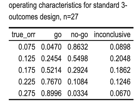
Based on the results above, for the inconclusive decision:
r=4.
With this information, we can use dual criterion to test its characteristics:1
2
3
4
5
6
7
8
9
10
11
12
13
14
15
16
17
18
19
20
21
22alpha <- 0.05
dv <- 0.175
nv <- 0.075
ssn <- 27
beta_a=0.0811
beta_b=1
result1 <- matrix(NA,nrow = 3,ncol=1)
r <- 4
# statistical significance and posterior median
rand <- rbeta(10000,beta_a+r,beta_b+ssn-r)
sig <- mean(rand>=nv)
med <- median(rand)
result1[1,1] <- r
result1[2,1] <- sig
result1[3,1] <- med
df1 <- data.frame(result1)
row.names(df1) <- c("r","statsig","postmedian")
df1 %>%
kbl(caption = "minimum responders, n=27") %>%
kable_classic(full_width = F)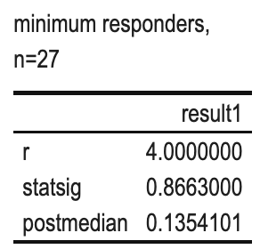
From the results, a NO-GO decision will be made, whereas the 3-outcome design results in an inconclusive outcome.