Sequential Enrichment Designs for Early Phase Clinical Trials (Reproducing Results)

This post reproduces the results from the presentation Sequential Enrichment Designs for Early Phase Clinical Trials.

Background

Study objective

  • PoC study of Drug A to evaluate its anti-tumor activity in gastric cancer

Endpoint

  • Objective response rate (ORR) Study population
  • All patients irrespective of status for biomarker of interest Y

Study design

  • Single-arm with biomarker of interest Y

Dual Criteria Design

  • Formal inclusion of statistical significance and clinical relevance in design:
  • Decide GO
    • Strong evidence: effect ≥ no effect or null value (NV)
    • Estimated effect ≥ decision value (DV)
  • DV : minimum effect with clinical relevance; not classical alternative hypothesis
    • Need discussion with nonstatisticians
  • Sample size requires consideration of DV
    • Adequate sample size is required to ensure statistical significance when clinical relevance observed
  • Need simulation to calculate design operating characteristics (e.g., type-I error, power)

Subpopulation Selection in Early Phase

Demand for a new design

  • A competitor Drug B failed for all-comers but show promising efficacy in patients with Y+ in post-hoc subgroup analysis

Goal

  • Assess activity of Drug A for all patients irrespective of biomarker status
  • If it is not active for all patients, assess activity of Drug A for Y+ patients

Single-stage Design with Population Selection

Brief Description

  • Study populations All-comers (F) = Y+ patients + Y- patients

  • Bayesian triplet criterion for all-comers

    1. Pr(ORR (F) ≥ 16% | data) ≥ 0.975
    2. Posterior median (F) ≥ 24%
    3. Pr(ORR (Y-) ≥ 16% | data) ≥ 0.75 (activity assurance in Y- patients)

The third criteria ensures that the effect of Drug A in F is not solely driven by Y+

  • Bayesian dual criteria for Y+ patients
    1. Pr(ORR (Y+) ≥ 16% | data) ≥ 0.95
    2. Posterior median (Y+) ≥ 24%
  • Minimum sample size (SSmin) All-comers: 87 (with number of responders ≥21) Y+ patients: 58 (with number of responders ≥14)

Sample size bigger than SSmin ensures statistical significance when clinical relevance is observed

Figure 1: Flow Chart for Single-stage Enrichment Design
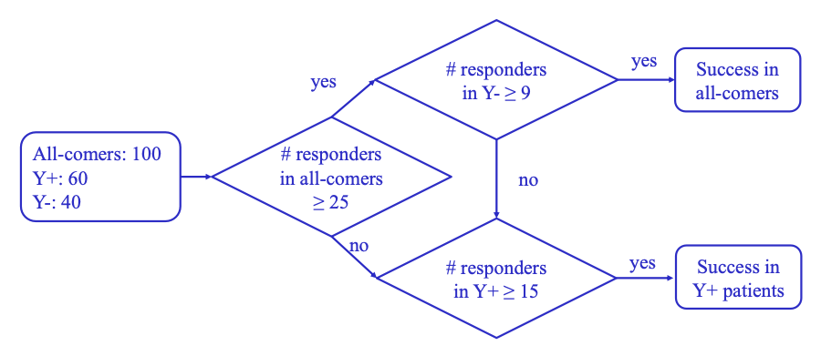
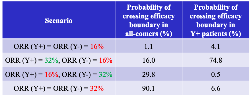
Figure 2: OC for One-stage Enrichment Design
Main Body of R Code

1
2
3
4
5
6
7
8
9
10
11
12
13
14
15
16
17
18
19
20
21
22
23
24
25
26
27
28
29
30
31
32
33
34
35
36
37
38
39
40
41
42
43
44
45
46
47
48
49
50
51
52
53
54
55
56
57
58
59
60
61
62
63
64
65
66
67
68
69
70
71
72
73
74
75
76
77
78
79
80
81
82
83
84
85
86
87
88
89
90
91
92
93
94
95
96
97
98
99
100
101
102
103
104
105
106
107
108
109
110
111
112
113
114
115
116
117
118
119
120
121
122
123
124
125
126
127
128
129
130
131
132
133
134
135
136
137
138
139
140
141
142
143
144
145
146
147
148
149
150
151
152
153
154
155
156
157
158
159
160
161
162
163
164
165
166
167
168
169
170
171
172
173
174
175
176
177
178
179
180
181
182
183
184
185
186
187
188
189
190
191
192
193
194
195
196
197
198
199
200
201
202
203
204
205
206
207
208
209
210
211
212
213
214
215
216
217
218
219
220
221
222
223
224
225
226
227
228
229
230
231
232
233
234
235
236
237
238
239
240
241
242
243
244
245
246
247
248
249
250
251
252
253
254
255
#######################################################################
#
# Pfizer- One Stage Enrichment Designs for Early Phase Clinical Trials
#
#######################################################################

library(dplyr)
library(ggplot2)
library(Rcpp)
library(stargazer) # 给txt输出排版用的包

start_time <- Sys.time()

#-*-*-*-*-*-*-*-*-*-*-*-*-*-*-*-*-*-*-*-*-*-*-*-*
# 0: 导入计算后验的c++外部函数
#-*-*-*-*-*-*-*-*-*-*-*-*-*-*-*-*-*-*-*-*-*-*-*-*

sourceCpp('function_cpp.cpp')

#-*-*-*-*-*-*-*-*-*-*-*-*-*-*-*-*-*-*-*-*-*-*-*-*
# 主程序1: 寻找Minimum sample size - Figure 1
#-*-*-*-*-*-*-*-*-*-*-*-*-*-*-*-*-*-*-*-*-*-*-*-*

nv = 0.16
statsig = 0.975
clinicalsig = 0.75
postmed = 0.24
positivestatsig = 0.95
maxsamplesize = 110 #我们能接受的样本量的上限,但是设太低可能会找不到
samplesize_start = 30 #实际应用中,总不可能样本量从1开始的
maxresponse = 25 #实际应用中可能出现的最高的responders数量?

beta_a = 0.1904762 #先验变化会对minimum sample size有影响,就算是无信息先验
beta_b = 1

totalrow = (maxsamplesize-samplesize_start+1)*(maxresponse)

df <- as.data.frame(responsegate(maxresponse = maxresponse,
samplesizestart = samplesize_start,
maxsamplesize = maxsamplesize,
a = beta_a,
b = beta_b,
nv = nv,
positivestatsig = positivestatsig,
statsig = statsig,
postmed = postmed))

colnames(df) <- c("r","n","significance","postmedian","justmedfl","bothfl","tripfl","group")

# 删去不满足任何标准的行记录
df_cc <- filter(df,justmedfl==1 | bothfl==1 | tripfl==1)

# recode
df_cc <- df_cc %>%
mutate(group=recode(group,'2'="full",'3'="positive only",'4'="n/a"))

## 最小样本量逻辑:按照n分组,找到最小的那个significance,因为一旦满足当前的要求,
## 则对于这个n,比当前significance对应的r更大的r,它的significance肯定更高

df_cc_plot <- df_cc %>%
group_by(n) %>%
slice(which.min(significance))

# 可视化最小样本量
text_y <- min(df_cc_plot$significance)+0.002
min_y <- min(df_cc_plot$significance)
max_y <- max(df_cc_plot$significance)

p <- ggplot(data=df_cc_plot, mapping = aes(x=n,y=significance)) +
geom_point(aes(color = factor(group)), size = 2, shape=17) +
geom_hline(yintercept=positivestatsig, linetype="dashed", color = "orange") +
geom_hline(yintercept=statsig, linetype="dashed", color = "orange") +
geom_vline(xintercept=58, linetype="dashed", color = "black") +
geom_vline(xintercept=87, linetype="dashed", color = "black") +
annotate(geom="text", x=58+7, y=text_y, label= "r/n=15/58") +
annotate(geom="text", x=87+7, y=text_y, label= "r/n=22/87") +
scale_y_continuous(name="Statistical Significance", limits=c(min_y, max_y))+
labs(color="Group") +
theme_classic()
p

#-*-*-*-*-*-*-*-*-*-*-*-*-*-*-*-*-*-*-*-*-*-*-*-*
# 主程序2: 评估设计的OC
#-*-*-*-*-*-*-*-*-*-*-*-*-*-*-*-*-*-*-*-*-*-*-*-*

allcomers = 100
y_plus = 60
y_minus = allcomers-y_plus

# 基于100人总样本量,60人Y+,40人Y-,去数据集df_cc_plot里寻找对应的responder gate
responder_gate <- df_cc_plot %>%
filter(n == allcomers | n==y_plus | n==y_minus) %>%
select(c(r,n))

full_gate <- responder_gate[which(responder_gate$n==allcomers),1]$r
y_plus_gate <- responder_gate[which(responder_gate$n==y_plus),1]$r

# Y-的responders
Y_minus_significance <- 0.75

y_minus_dec <- df %>% filter(n==y_minus & significance>=Y_minus_significance)

y_minus_dec2 <- y_minus_dec %>%
slice(which.min(r))
y_minus_gate <- y_minus_dec2$r

# 不同场景的orr假设
## 1
orr_plus_1 <- 0.16
orr_minus_1 <- 0.16
## 2
orr_plus_2 <- 0.32
orr_minus_2 <- 0.16
## 3
orr_plus_3 <- 0.16
orr_minus_3 <- 0.32
## 4
orr_plus_4 <- 0.32
orr_minus_4 <- 0.32

simoc <- function(orr_plus,
orr_minus,
allcomers,
y_plus,
y_minus,
full_gate,
y_plus_gate,
y_minus_gate,
rep){

# 初始化模拟矩阵
simmat <- data.frame(orr_plus=rep(NA,rep),
orr_minus=rep(NA,rep),
allcomers=rep(NA,rep),
y_plus=rep(NA,rep),
y_minus=rep(NA,rep),
full_gate=rep(NA,rep),
y_plus_gate=rep(NA,rep),
y_plus_responders=rep(NA,rep),
full_responders=rep(NA,rep),
succ_full=rep(FALSE,rep),
succ_y_pos=rep(FALSE,rep))

for (row in 1:rep){
resp_y_plus <- sum(rbinom(y_plus,1,orr_plus))
resp_y_minus <- sum(rbinom(y_minus,1,orr_minus))
total_resp <- resp_y_minus+resp_y_plus

#决策 - 怎么避免重复书写? if 太多了
if (total_resp >= full_gate){
if (resp_y_minus >= y_minus_gate){
simmat[row,"succ_full"] <- TRUE
} else {
if (resp_y_plus >= y_plus_gate){
simmat[row,"succ_y_pos"] <- TRUE
}
}
} else{
if (resp_y_plus >= y_plus_gate){
simmat[row,"succ_y_pos"] <- TRUE
}
}

# simmat赋值
simmat[row,"orr_plus"] <- orr_plus
simmat[row,"orr_minus"] <- orr_minus
simmat[row,"allcomers"] <- allcomers
simmat[row,"y_plus"] <- y_plus
simmat[row,"y_minus"] <- y_minus
simmat[row,"full_gate"] <- full_gate
simmat[row,"y_plus_gate"] <- y_plus_gate
simmat[row,"y_plus_responders"] <- resp_y_plus
simmat[row,"full_responders"] <- total_resp
}

return(simmat)
}

rep = 12000

scen1 <- simoc(orr_plus_1,
orr_minus_1,
allcomers,
y_plus,
y_minus,
full_gate,
y_plus_gate,
y_minus_gate,
rep)

scen2 <- simoc(orr_plus_2,
orr_minus_2,
allcomers,
y_plus,
y_minus,
full_gate,
y_plus_gate,
y_minus_gate,
rep)

scen3 <- simoc(orr_plus_3,
orr_minus_3,
allcomers,
y_plus,
y_minus,
full_gate,
y_plus_gate,
y_minus_gate,
rep)

scen4 <- simoc(orr_plus_4,
orr_minus_4,
allcomers,
y_plus,
y_minus,
full_gate,
y_plus_gate,
y_minus_gate,
rep)

# 汇报结果 - 与壁报的Figure 6.2 OC for One stage Enrichment Design 对比
result <- data.frame(scenario=rep(NA,4),
prob_eff_full=rep(NA,4),
prob_eff_positive=rep(NA,4))

result[1,"scenario"] <- "ORR (Y+) = ORR (Y-) = 16%"
result[2,"scenario"] <- "ORR (Y+) = 32%, ORR (Y-) = 16%"
result[3,"scenario"] <- "ORR (Y+) = 16%, ORR (Y-) = 32%"
result[4,"scenario"] <- "ORR (Y+) = ORR (Y-) = 32%"


result[1,"prob_eff_full"] <- mean(scen1$succ_full)*100
result[2,"prob_eff_full"] <- mean(scen2$succ_full)*100
result[3,"prob_eff_full"] <- mean(scen3$succ_full)*100
result[4,"prob_eff_full"] <- mean(scen4$succ_full)*100

result[1,"prob_eff_positive"] <- mean(scen1$succ_y_pos)*100
result[2,"prob_eff_positive"] <- mean(scen2$succ_y_pos)*100
result[3,"prob_eff_positive"] <- mean(scen3$succ_y_pos)*100
result[4,"prob_eff_positive"] <- mean(scen4$succ_y_pos)*100

# 评估程序运行时间
end_time <- Sys.time()
end_time-start_time

# 输出TXT
stargazer(result,
title = "OC for One stage Enrichment Design",
summary = FALSE,
rownames = FALSE,
type = "text",
align = TRUE,
out = "单阶段富集设计OC.txt",
notes = paste0("程序运行用时",as.character.Date(end_time-start_time),", 可对比辉瑞壁报Figure 6.2"),
notes.align = "l")

Utility Function

1
2
3
4
5
6
7
8
9
10
11
12
13
14
15
16
17
18
19
20
21
22
23
24
25
26
27
28
29
30
31
32
33
34
35
36
37
38
39
40
41
42
43
44
45
46
47
48
49
50
51
52
53
54
55
#include <Rcpp.h>
using namespace Rcpp;

// [[Rcpp::export]]
NumericVector responsegate(int maxresponse,int samplesizestart,int maxsamplesize,double a,double b,double nv,double positivestatsig,double statsig,double postmed){
// Creating object
int row,totalrow,f1,f2,f3;
double med,sig;
totalrow = (maxsamplesize-samplesizestart+1)*(maxresponse);
NumericMatrix df(totalrow,8);
row = 0;
// using loop to construct response matrix
for(int r = 1; r <= maxresponse; ++r) {
for(int n = samplesizestart; n <= maxsamplesize; ++n) {
// generate beta random numbers
NumericVector rand = Rcpp::rbeta( 100000, a+r, b+n-r);
// compare to nv
LogicalVector logicnv = rand >= nv;
sig= mean(logicnv);
med = median(rand);
// output
df(row,0) = r;
df(row,1) = n;
df(row,2)=sig;
df(row,3)=med;
// decision flag
f1=0;
f2=0;
f3=0;
if (sig<positivestatsig && med>=postmed){
df(row,4)=1;
f1=1;
};
if (sig>=positivestatsig && med>=postmed && sig<statsig){
df(row,5)=1;
f2=1;
};
if (sig>=statsig && med>=postmed){
df(row,6)=1;
f3=1;
};
// 2-full,3-positive only,4-n/a
if (f3==1){
df(row,7) = 2;
} else if(f2==1){
df(row,7) = 3;
} else if (f1==1){
df(row,7) = 4;
}
row++;
}
}
return df;
}

OC

1
2
3
4
5
6
7
8
9
10
OC for One stage Enrichment Design
==============================================================
scenario prob_eff_full prob_eff_positive
--------------------------------------------------------------
ORR (Y+) = ORR (Y-) = 16% 0.983 4.067
ORR (Y+) = 32%, ORR (Y-) = 16% 16.150 74.242
ORR (Y+) = 16%, ORR (Y-) = 32% 29.567 0.467
ORR (Y+) = ORR (Y-) = 32% 90.350 6.158
--------------------------------------------------------------
程序运行用时1.095885 mins, 可对比辉瑞壁报Figure 6.2

Two-stage Design with Adaptive Population Enrichment

Brief Description

  • Sequential enrichment
    • Use probability of success (POS) at interim to allow early stopping for futility.
  • Use POS for interim decision making
    • POS(F): PP(posterior median (F) ≥ 24% at final analysis | interim data); PP=predictive probability
    • POS(Y+): PP(posterior median (Y+) ≥ 24% at final analysis | interim data)
    • POS(Y-): PP (Pr(ORR (Y-) ≥ 16% | data) ≥ 0.75 at final analysis | interim data)
  • Interim decision rules
    • Continue with F: POS(F) ≥ 10% and POS(Y-) ≥ 10%
    • Continue with Y+: POS(F) ≥ 10% but POS(Y-) < 10% and POS(Y+) ≥ 10% OR
    • POS(F) < 10% but POS(Y+) ≥ 10%

Otherwise stop for futility.

Figure 3: Flow Chart for Sequential Enrichment Design

Figure 4: Interim OC for Sequential Enrichment Design
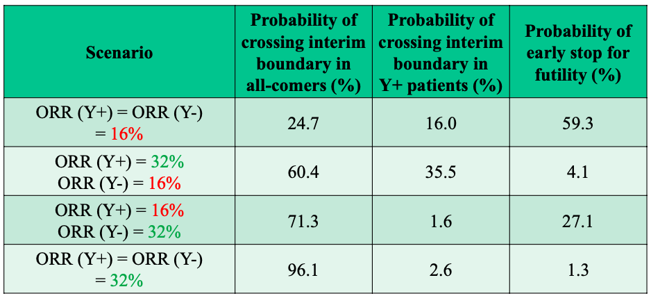
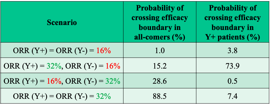
Figure 5: Final OC for Sequential Enrichment Design
Main Body of R Code

1
2
3
4
5
6
7
8
9
10
11
12
13
14
15
16
17
18
19
20
21
22
23
24
25
26
27
28
29
30
31
32
33
34
35
36
37
38
39
40
41
42
43
44
45
46
47
48
49
50
51
52
53
54
55
56
57
58
59
60
61
62
63
64
65
66
67
68
69
70
71
72
73
74
75
76
77
78
79
80
81
82
83
84
85
86
87
88
89
90
91
92
93
94
95
96
97
98
99
100
101
102
103
104
105
106
107
108
109
110
111
112
113
114
115
116
117
118
119
120
121
122
123
124
125
126
127
128
129
130
131
132
133
134
135
136
137
138
139
140
141
142
143
144
145
146
147
148
149
150
151
152
153
154
155
156
157
158
159
160
161
162
163
164
165
166
167
168
169
170
171
172
173
174
175
176
177
178
179
180
181
182
183
184
185
186
187
188
189
190
191
192
193
194
195
196
197
198
199
200
201
202
203
204
205
206
207
208
209
210
211
212
213
214
215
216
217
218
219
220
221
222
223
224
225
226
227
228
229
230
231
232
233
234
235
236
237
238
239
240
241
242
243
244
245
246
247
248
249
250
251
252
253
254
255
256
257
258
259
260
261
262
263
264
265
266
267
268
269
270
271
272
273
274
275
276
277
278
279
280
281
282
283
284
285
286
287
288
289
290
291
292
293
294
295
296
297
298
299
300
301
302
303
304
305
306
307
308
309
310
311
312
313
314
315
316
317
318
319
320
321
322
323
324
325
326
327
328
329
330
331
332
333
334
335
336
337
338
339
340
341
342
343
344
345
346
347
348
349
350
351
352
353
354
355
356
357
358
359
360
361
362
363
364
365
366
367
368
369
370
371
372
373
374
375
376
377
378
379
380
381
382
383
384
385
386
387
388
389
390
391
392
393
394
395
396
397
398
399
400
401
402
403
404
405
406
407
408
409
410
411
412
413
414
415
416
417
418
419
420
421
422
423
424
425
426
427
428
429
430
431
432
433
434
435
436
437
438
439
440
441
442
443
444
445
446
447
448
449
450
451
452
453
454
455
456
457
458
459
460
461
462
463
464
465
466
467
468
469
470
471
472
473
474
475
476
477
478
479
480
#######################################################################
#
# Pfizer- Sequential Enrichment Designs for Early Phase Clinical Trials
#
#######################################################################

library(dplyr)
library(ggplot2)
library(Rcpp)
library(reshape2)
library(stargazer) # 给txt输出排版用的包

start_time <- Sys.time()

#-*-*-*-*-*-*-*-*-*-*-*-*-*-*-*-*-*-*-*-*-*-*-*-*
# 0: 导入计算后验的c++外部函数
#-*-*-*-*-*-*-*-*-*-*-*-*-*-*-*-*-*-*-*-*-*-*-*-*

sourceCpp('function_cpp.cpp')
sourceCpp('predprobMedian.cpp')
sourceCpp('predprobPosterior.cpp')

#-*-*-*-*-*-*-*-*-*-*-*-*-*-*-*-*-*-*-*-*-*-*-*-*
# 主程序1: 寻找中期分析的决策边界
#-*-*-*-*-*-*-*-*-*-*-*-*-*-*-*-*-*-*-*-*-*-*-*-*

# 先验
beta_a = 0.1904762 #a/a+b=0.16倒推,先验变化会对minimum sample size有影响,就算是无信息先验
beta_b = 1

# 双标准决策中的边界
postmed = 0.24
nv = 0.16
clinicalsig = 0.75
pp_thres = 0.1

# 搜索的responders上限
max_responders <- 20

# 第一阶段full人群的样本量和final阶段full人群样本量,用来算PP
full_n1 <- 50
full_n_total <- 100
# 第一阶段Y+人群的样本量和final阶段Y+人群样本量,用来算PP
y_plus_n1 <- 30
y_plus_n_total <- 60
# 第一阶段Y-人群的样本量和final阶段Y-人群样本量,用来算PP
y_minus_n1 <- 20
y_minus_n_total <- 40

# 设置向量来收集full/Y+/Y-在期中的时候PP的结果
r_vec <- seq(1,max_responders,1)
full_succ_vec <- rep(NA,max_responders)
y_minus_succ_vec <- rep(NA,max_responders)
y_plus_succ_vec <- rep(NA,max_responders)

for (r in 0:max_responders){
full_pp <- predprobMedian(r,full_n1,full_n_total,beta_a,beta_b,postmed)
y_minus_pp <- predprobPosterior(r,y_minus_n1,y_minus_n_total,beta_a,beta_b,nv,clinicalsig)
y_plus_pp <- predprobMedian(r,y_plus_n1,y_plus_n_total,beta_a,beta_b,postmed)

# collect result
full_succ_vec[r] <- full_pp
y_minus_succ_vec[r] <- y_minus_pp
y_plus_succ_vec[r] <- y_plus_pp

# package result
result_df <- data.frame(r=r_vec,
fullpp=full_succ_vec,
yminuspp=y_minus_succ_vec,
ypluspp=y_plus_succ_vec)
}

result_df_t <- melt(result_df,id.vars = "r",variable.name = "population_pp")
result_df_t <- result_df_t %>% filter(!is.na(value))

p <- ggplot(data=result_df_t, mapping = aes(x=r,y=value)) +
geom_point(aes(color = factor(population_pp), shape=factor(population_pp)), size = 3) +
geom_hline(yintercept=clinicalsig, linetype="dotted", color = "orange",lwd=1) +
geom_hline(yintercept=pp_thres, linetype="dotted", color = "orange",lwd=1) +
# geom_vline(xintercept=58, linetype="dashed", color = "black") +
# geom_vline(xintercept=87, linetype="dashed", color = "black") +
scale_y_continuous(name="Predictive Probability")+
scale_x_continuous(name="#responders",breaks = seq(1,max_responders,1))+
labs(color="Group",shape="Group") +
theme(panel.background = element_rect(fill = NA),
panel.border = element_rect(linetype = "solid", fill = NA),
panel.grid.major.x = element_line(colour = "grey70",linetype = "longdash"))
p

#-*-*-*-*-*-*-*-*-*-*-*-*-*-*-*-*-*-*-*-*-*-*-*-*
# 主程序1.5.1: 第一阶段的决策边界
#-*-*-*-*-*-*-*-*-*-*-*-*-*-*-*-*-*-*-*-*-*-*-*-*

# 打印决策边界
result_df_t_decision <- result_df_t %>%
mutate(gt10=ifelse(value>0.1,TRUE,FALSE),
gt75=ifelse(value>0.1,TRUE,FALSE))

### Continue with F:POS(F) ≥ 10% and POS(Y-) ≥ 10%,能同时满足这两个条件
### 从上面的图中可以看出,当full人群的中期条件满足(50人里观察到10个full人群responders),此时去检查y-人群,responders>=3时可以满足Full期中的决策边界
F_dec <- result_df_t_decision %>%
filter(population_pp %in% c("fullpp","yminuspp") & value >= 0.1) %>%
group_by(population_pp) %>%
slice(which.min(r))
F_dec_r <- max(F_dec$r)
cat("The Go decision for full population is responders >= ",F_dec_r)

### Continue with Y+
### 从上面的图中可以看出,当full人群的中期条件满足(50人里观察到10个full人群responders),此时去检查y-人群,responders>=3时可以满足Full期中的决策边界
### condition1: 药物在full人群展示出效果,Y-无效,Y+人群有效,拓展至Y+富集
### condition2: enrichment定义,药物在full人群展示不出效果,Y+人群有效,拓展至Y+富集
y_plus_dec <- result_df %>%
mutate(cond1 = ifelse(fullpp>=0.1 & yminuspp<0.1 & ypluspp>=0.1,TRUE,FALSE),
cond2 = ifelse(fullpp<0.1 & ypluspp>=0.1,TRUE,FALSE),
overall = cond1 | cond2)

y_plus_dec2 <- y_plus_dec %>%
filter(overall == TRUE) %>%
slice(which.min(r))

y_plus_dec_r <- max(y_plus_dec2$r)
cat("The Go decision for Y+ population is responders >= ",y_plus_dec_r)

### Continue with Y- if it continues with Full
y_minus_dec <- result_df %>%
mutate(cond1 = ifelse(yminuspp>=0.1,TRUE,FALSE))

y_minus_dec2 <- y_minus_dec %>%
filter(cond1 == TRUE) %>%
slice(which.min(r))

y_minus_dec_r <- max(y_minus_dec2$r)
cat("The Go decision for Y- population is responders >= ",y_minus_dec_r)

#-*-*-*-*-*-*-*-*-*-*-*-*-*-*-*-*-*-*-*-*-*-*-*-*
# 主程序1.5.2: 第二阶段的决策边界
#-*-*-*-*-*-*-*-*-*-*-*-*-*-*-*-*-*-*-*-*-*-*-*-*

finalstage.df <- as.data.frame(responsegate(maxresponse = 30,
samplesizestart = 40,
maxsamplesize = 100,
a = beta_a,
b = beta_b,
nv = nv,
positivestatsig = 0.95,
statsig = 0.975,
postmed = postmed))
colnames(finalstage.df) <- c("r","n","significance","postmedian","justmedfl","bothfl","tripfl","group")

# 删去不满足任何标准的行记录
finalstage.df2 <- filter(finalstage.df,justmedfl==1 | bothfl==1 | tripfl==1)

# recode
finalstage.df2 <- finalstage.df2 %>%
mutate(group=recode(group,'2'="full",'3'="positive only",'4'="n/a"))

## 最小样本量逻辑:按照n分组,找到最小的那个significance,因为一旦满足当前的要求,
## 则对于这个n,比当前significance对应的r更大的r,它的significance肯定更高

finalstage.df3 <- finalstage.df2 %>%
group_by(n) %>%
slice(which.min(significance))

allcomers = full_n_total
y_plus = y_plus_n_total
y_minus = allcomers-y_plus

# 基于100人总样本量,60人Y+,40人Y-,去数据集df_cc_plot里寻找对应的responder gate
responder_gate_final <- finalstage.df3 %>%
filter(n == allcomers | n==y_plus | n==y_minus) %>%
select(c(r,n))

full_FA_gate <- responder_gate_final[which(responder_gate_final$n==allcomers),1]$r
y_plus_FA_gate <- responder_gate_final[which(responder_gate_final$n==y_plus),1]$r

#最后阶段Y-的responder gate
y_minus_dec_final <- finalstage.df %>% filter(n==y_minus_n_total & significance>=0.75)

y_minus_dec2_final <- y_minus_dec_final %>%
slice(which.min(r))
y_minus_FA_gate <- y_minus_dec2_final$r
#-*-*-*-*-*-*-*-*-*-*-*-*-*-*-*-*-*-*-*-*-*-*-*-*
# 主程序2: 评估设计的OC
#-*-*-*-*-*-*-*-*-*-*-*-*-*-*-*-*-*-*-*-*-*-*-*-*

# 不同场景的orr假设
## 1
orr_plus_1 <- 0.16
orr_minus_1 <- 0.16
## 2
orr_plus_2 <- 0.32
orr_minus_2 <- 0.16
## 3
orr_plus_3 <- 0.16
orr_minus_3 <- 0.32
## 4
orr_plus_4 <- 0.32
orr_minus_4 <- 0.32

# 人数假设
allcomers_ia <- full_n1
y_plus_ia <- y_plus_n1
y_minus_ia <- y_minus_n1
allcomers_overall <- full_n_total
y_plus_overall <- y_plus_n_total
y_minus_overall <- y_minus_n_total
rep <- 5000

# 设置responder threshold,从上面的试验设计中得来
full_IA_gate <- F_dec_r
full_FA_gate <- full_FA_gate

y_plus_IA_gate <- y_plus_dec_r
y_plus_FA_gate <- y_plus_FA_gate

y_minus_IA_gate <- y_minus_dec_r
y_minus_FA_gate <- y_minus_FA_gate

simseqoc <- function(orr_plus,
orr_minus,
allcomers_ia,
y_plus_ia,
y_minus_ia,
allcomers_overall,
y_plus_overall,
y_minus_overall,
full_IA_gate,
full_FA_gate,
y_plus_IA_gate,
y_plus_FA_gate,
y_minus_IA_gate,
y_minus_FA_gate,
rep){

# 初始化模拟矩阵, s1: stage 1; s2: stage 2; overall=s1+s2
simmat <- data.frame(orr_plus=rep(NA,rep),
orr_minus=rep(NA,rep),
allcomers_s1=rep(NA,rep),
y_plus_s1=rep(NA,rep),
y_minus_s1=rep(NA,rep),
allcomers_s2=rep(NA,rep),
y_plus_s2=rep(NA,rep),
y_minus_s2=rep(NA,rep),
full_gate_s1=rep(NA,rep),
y_plus_gate_s1=rep(NA,rep),
y_minus_gate_s1=rep(NA,rep),
full_gate_s2=rep(NA,rep),
y_plus_gate_s2=rep(NA,rep),
y_minus_gate_s2=rep(NA,rep),
y_plus_responders_s1=rep(NA,rep),
full_responders_s1=rep(NA,rep),
y_plus_responders_overall=rep(NA,rep),
full_responders_overall=rep(NA,rep),
succ_ia_full=rep(FALSE,rep),
succ_ia_y_pos=rep(FALSE,rep),
early_stop=rep(FALSE,rep),
succ_overall_full=rep(FALSE,rep),
succ_overall_y_pos=rep(FALSE,rep))

for (row in 1:rep){

# 产生overall样本量的随机数
y_plus_data <- rbinom(y_plus_overall,1,orr_plus)
y_minus_data <- rbinom(y_minus_overall,1,orr_minus)

# 切割向量,生成中期分析数据集
y_plus_ia_data <- y_plus_data[1:y_plus_ia]
y_minus_ia_data <- y_minus_data[1:y_minus_ia]

# 计算IA 及 overall分别有多少responders
## IA
resp_y_plus_ia <- sum(y_plus_ia_data)
resp_y_minus_ia <- sum(y_minus_ia_data)
total_resp_ia <- resp_y_plus_ia+resp_y_minus_ia
## OVERALL
resp_y_plus_overall <- sum(y_plus_data)
resp_y_minus_overall <- sum(y_minus_data)
total_resp_overall <- resp_y_plus_overall+resp_y_minus_overall

#决策 - 怎么避免重复书写? if 太多了
## 先设置不同IA前进方向/最终结果判断的flag,否则IF太多了很乱
IA_go_withF <- FALSE
IA_go_withYPlus <- FALSE
IA_ET <- FALSE
SUCC_F <- FALSE
SUCC_YPlus <- FALSE
FA_FAIL <- FALSE
## S1的决策部分
if (total_resp_ia>=full_IA_gate){
if (resp_y_minus_ia>=y_minus_IA_gate){
IA_go_withF <- TRUE
} else if (resp_y_minus_ia<y_minus_IA_gate){
if (resp_y_plus_ia>=y_plus_IA_gate){
IA_go_withYPlus <- TRUE
} else {
IA_ET <- TRUE
}
}
} else if (total_resp_ia<full_IA_gate){
if (resp_y_plus_ia>=y_plus_IA_gate){
IA_go_withYPlus <- TRUE
} else {
IA_ET <- TRUE
}
}
## S2的决策部分
### Full
if (IA_go_withF==TRUE){
if (total_resp_overall >= full_FA_gate){
if (resp_y_minus_overall >= y_minus_FA_gate){
SUCC_F <- TRUE
} else {
if (resp_y_plus_overall >= y_plus_FA_gate){
SUCC_YPlus <- TRUE
}
}
} else{
if (resp_y_plus_overall >= y_plus_FA_gate){
SUCC_YPlus <- TRUE
}
}
}
### Y+
if (IA_go_withF!=TRUE & IA_go_withYPlus==TRUE){
if (resp_y_plus_overall >= y_plus_FA_gate){
SUCC_YPlus <- TRUE
} else {
FA_FAIL <- TRUE
}
}


# simmat赋值
simmat[row,"orr_plus"] <- orr_plus
simmat[row,"orr_minus"] <- orr_minus
simmat[row,"allcomers_s1"] <- allcomers_ia
simmat[row,"y_plus_s1"] <- y_plus_ia
simmat[row,"y_minus_s1"] <- y_minus_ia
simmat[row,"allcomers_s2"] <- allcomers_overall
simmat[row,"y_plus_s2"] <- y_plus_overall
simmat[row,"y_minus_s2"] <- y_minus_ia
simmat[row,"full_gate_s1"] <- full_IA_gate
simmat[row,"y_plus_gate_s1"] <- y_plus_IA_gate
simmat[row,"y_minus_gate_s1"] <- y_minus_IA_gate
simmat[row,"full_gate_s2"] <- full_FA_gate
simmat[row,"y_plus_gate_s2"] <- y_plus_FA_gate
simmat[row,"y_minus_gate_s2"] <- y_minus_FA_gate
simmat[row,"y_plus_responders_s1"] <- resp_y_plus_ia
simmat[row,"full_responders_s1"] <- total_resp_ia
simmat[row,"y_plus_responders_overall"] <- resp_y_plus_overall
simmat[row,"full_responders_overall"] <- total_resp_overall
simmat[row,"succ_ia_full"] <- IA_go_withF
simmat[row,"succ_ia_y_pos"] <- IA_go_withYPlus
simmat[row,"early_stop"] <- IA_ET
simmat[row,"succ_overall_full"] <- SUCC_F
simmat[row,"succ_overall_y_pos"] <- SUCC_YPlus

}

return(simmat)
}

rep = 5000

scen1 <- simseqoc(orr_plus_1,
orr_minus_1,
allcomers_ia,
y_plus_ia,
y_minus_ia,
allcomers_overall,
y_plus_overall,
y_minus_overall,
full_IA_gate,
full_FA_gate,
y_plus_IA_gate,
y_plus_FA_gate,
y_minus_IA_gate,
y_minus_FA_gate,
rep)

scen2 <- simseqoc(orr_plus_2,
orr_minus_2,
allcomers_ia,
y_plus_ia,
y_minus_ia,
allcomers_overall,
y_plus_overall,
y_minus_overall,
full_IA_gate,
full_FA_gate,
y_plus_IA_gate,
y_plus_FA_gate,
y_minus_IA_gate,
y_minus_FA_gate,
rep)

scen3 <- simseqoc(orr_plus_3,
orr_minus_3,
allcomers_ia,
y_plus_ia,
y_minus_ia,
allcomers_overall,
y_plus_overall,
y_minus_overall,
full_IA_gate,
full_FA_gate,
y_plus_IA_gate,
y_plus_FA_gate,
y_minus_IA_gate,
y_minus_FA_gate,
rep)

scen4 <- simseqoc(orr_plus_4,
orr_minus_4,
allcomers_ia,
y_plus_ia,
y_minus_ia,
allcomers_overall,
y_plus_overall,
y_minus_overall,
full_IA_gate,
full_FA_gate,
y_plus_IA_gate,
y_plus_FA_gate,
y_minus_IA_gate,
y_minus_FA_gate,
rep)

# 汇报结果 - 与壁报的Figure 6.2 OC for One stage Enrichment Design 对比
result <- data.frame(scenario=rep(NA,4),
prob_eff_full_IA=rep(NA,4),
prob_eff_positive_IA=rep(NA,4),
prob_ET_IA=rep(NA,4),
prob_eff_full_FA=rep(NA,4),
prob_eff_positive_FA=rep(NA,4))

result[1,"scenario"] <- "ORR (Y+) = ORR (Y-) = 16%"
result[2,"scenario"] <- "ORR (Y+) = 32%, ORR (Y-) = 16%"
result[3,"scenario"] <- "ORR (Y+) = 16%, ORR (Y-) = 32%"
result[4,"scenario"] <- "ORR (Y+) = ORR (Y-) = 32%"


result[1,"prob_eff_full_IA"] <- mean(scen1$succ_ia_full)*100
result[2,"prob_eff_full_IA"] <- mean(scen2$succ_ia_full)*100
result[3,"prob_eff_full_IA"] <- mean(scen3$succ_ia_full)*100
result[4,"prob_eff_full_IA"] <- mean(scen4$succ_ia_full)*100

result[1,"prob_eff_positive_IA"] <- mean(scen1$succ_ia_y_pos)*100
result[2,"prob_eff_positive_IA"] <- mean(scen2$succ_ia_y_pos)*100
result[3,"prob_eff_positive_IA"] <- mean(scen3$succ_ia_y_pos)*100
result[4,"prob_eff_positive_IA"] <- mean(scen4$succ_ia_y_pos)*100

result[1,"prob_ET_IA"] <- mean(scen1$early_stop)*100
result[2,"prob_ET_IA"] <- mean(scen2$early_stop)*100
result[3,"prob_ET_IA"] <- mean(scen3$early_stop)*100
result[4,"prob_ET_IA"] <- mean(scen4$early_stop)*100

result[1,"prob_eff_full_FA"] <- mean(scen1$succ_overall_full)*100
result[2,"prob_eff_full_FA"] <- mean(scen2$succ_overall_full)*100
result[3,"prob_eff_full_FA"] <- mean(scen3$succ_overall_full)*100
result[4,"prob_eff_full_FA"] <- mean(scen4$succ_overall_full)*100

result[1,"prob_eff_positive_FA"] <- mean(scen1$succ_overall_y_pos)*100
result[2,"prob_eff_positive_FA"] <- mean(scen2$succ_overall_y_pos)*100
result[3,"prob_eff_positive_FA"] <- mean(scen3$succ_overall_y_pos)*100
result[4,"prob_eff_positive_FA"] <- mean(scen4$succ_overall_y_pos)*100

# 评估程序运行时间
end_time <- Sys.time()

# 打印到txt文件
stargazer(result,
title = "Interim & Final OC for Sequential Enrichment Design",
summary = FALSE,
rownames = FALSE,
type = "text",
align = TRUE,
out = "两阶段富集设计OC.txt",
notes = paste0("程序运行用时",as.character.Date(end_time-start_time),", 可对比辉瑞壁报Figure 8.2与Figure 8.3"),
notes.align = "l")

Utility Function

function_cpp.cpp

1
2
3
4
5
6
7
8
9
10
11
12
13
14
15
16
17
18
19
20
21
22
23
24
25
26
27
28
29
30
31
32
33
34
35
36
37
38
39
40
41
42
43
44
45
46
47
48
49
50
51
52
53
54
55
#include <Rcpp.h>
using namespace Rcpp;

// [[Rcpp::export]]
NumericVector responsegate(int maxresponse,int samplesizestart,int maxsamplesize,double a,double b,double nv,double positivestatsig,double statsig,double postmed){
// Creating object
int row,totalrow,f1,f2,f3;
double med,sig;
totalrow = (maxsamplesize-samplesizestart+1)*(maxresponse);
NumericMatrix df(totalrow,8);
row = 0;
// using loop to construct response matrix
for(int r = 1; r <= maxresponse; ++r) {
for(int n = samplesizestart; n <= maxsamplesize; ++n) {
// generate beta random numbers
NumericVector rand = Rcpp::rbeta( 100000, a+r, b+n-r);
// compare to nv
LogicalVector logicnv = rand >= nv;
sig= mean(logicnv);
med = median(rand);
// output
df(row,0) = r;
df(row,1) = n;
df(row,2)=sig;
df(row,3)=med;
// decision flag
f1=0;
f2=0;
f3=0;
if (sig<positivestatsig && med>=postmed){
df(row,4)=1;
f1=1;
};
if (sig>=positivestatsig && med>=postmed && sig<statsig){
df(row,5)=1;
f2=1;
};
if (sig>=statsig && med>=postmed){
df(row,6)=1;
f3=1;
};
// 2-full,3-positive only,4-n/a
if (f3==1){
df(row,7) = 2;
} else if(f2==1){
df(row,7) = 3;
} else if (f1==1){
df(row,7) = 4;
}
row++;
}
}
return df;
}

predprobMedian.cpp

1
2
3
4
5
6
7
8
9
10
11
12
13
14
15
16
17
18
19
20
21
22
23
24
25
26
27
28
29
30
#include <Rcpp.h>
using namespace Rcpp;


// [[Rcpp::export]]
double predprobMedian(int x, int n, int nmax, double alpha, double beta, double theta_t) {

double prob = 0.0;
double eps = std::numeric_limits<double>::epsilon();
double med;

for (int resp = 0; resp < nmax - n + 1; resp++) {
// --------------------------------------------------------
// --- use median instead of posterior in pfizer's settings
// --------------------------------------------------------
// generate beta random numbers
NumericVector rand = Rcpp::rbeta( 100000, alpha + x + resp, beta + nmax - x - resp);
med = median(rand);
if (med > theta_t || std::abs(med - theta_t) < eps) {
prob += exp(
R::lchoose(nmax - n, resp) +
R::lbeta(alpha + x + resp, beta + nmax - x - resp) -
R::lbeta(alpha + x, beta + n - x)
);
}
}

return prob;

}

predprobPosterior.cpp

1
2
3
4
5
6
7
8
9
10
11
12
13
14
15
16
17
18
19
20
21
22
23
#include <Rcpp.h>
using namespace Rcpp;


// [[Rcpp::export]]
double predprobPosterior(int x, int n, int nmax, double alpha, double beta, double p0, double theta_t){

double prob = 0.0;
double eps = std::numeric_limits<double>::epsilon();
double pxy;

for (int resp = 0; resp < nmax - n + 1; resp++) {
pxy = (1.0 - R::pbeta(p0, alpha + resp + x, beta + nmax - resp - x, 1, 0));
if (pxy > theta_t || std::abs(pxy - theta_t) < eps) {
prob += exp(
R::lchoose(nmax - n, resp) +
R::lbeta(alpha + resp + x, beta + nmax - resp - x) -
R::lbeta(alpha + x, beta + n - x)
);
}
}
return prob;
}

OC

1
2
3
4
5
6
7
8
9
10
11
12

Interim & Final OC for Sequential Enrichment Design
=====================================================================================================================
scenario prob_eff_full_IA prob_eff_positive_IA prob_ET_IA prob_eff_full_FA prob_eff_positive_FA
---------------------------------------------------------------------------------------------------------------------
ORR (Y+) = ORR (Y-) = 16% 24.280 16.360 59.360 1.060 4.080
ORR (Y+) = 32%, ORR (Y-) = 16% 59.740 35.800 4.460 14.780 73.860
ORR (Y+) = 16%, ORR (Y-) = 32% 70.980 1.640 27.380 28.160 0.540
ORR (Y+) = ORR (Y-) = 32% 96.020 2.620 1.360 88.340 8.040
---------------------------------------------------------------------------------------------------------------------
程序运行用时1.384589 mins, 可对比辉瑞壁报Figure 8.2与Figure 8.3

Appendix - Comparison of R & RCPP

1
2
3
4
5
6
7
8
9
10
11
12
13
14
15
16
17
18
19
20
21
22
23
24
25
26
27
28
29
30
31
32
33
34
35
36
37
38
39
40
41
42
43
44
45
46
47
48
49
50
51
52
53
54
55
56
57
58
59
60
61
62
63
64
65
66
67
68
69
70
71
72
library(Rcpp)
sourceCpp('function_cpp.cpp')

# Rcpp

start_time <- Sys.time()
aaa <- responsegate(maxresponse = 100,samplesizestart = 30,maxsamplesize = 200,a = 0.1904762,b = 1,nv = 0.16,positivestatsig = 0.95,statsig = 0.975,postmed = 0.24)
end_time <- Sys.time()

# R
start_time2 <- Sys.time()
nv = 0.16
statsig = 0.975
clinicalsig = 0.75
postmed = 0.24
positivestatsig = 0.95
maxsamplesize = 200 #我们能接受的样本量的上限,但是设太低可能会找不到
samplesize_start = 30 #实际应用中,总不可能样本量从1开始的
maxresponse = 100 #实际应用中可能出现的最高的responders数量?

beta_a = 0.1904762 #先验变化会对minimum sample size有影响,就算是无信息先验
beta_b = 1

totalrow = (maxsamplesize-samplesize_start+1)*(maxresponse)

# bothfl: for Bayesian dual criteria for Y+ patients
# tripfl: for Bayesian triplet criterion for all patients
df <- data.frame(r=rep(NA,totalrow),
n=rep(NA,totalrow),
significance=rep(NA,totalrow),
postmedian=rep(NA,totalrow),
justmedfl=rep(FALSE,totalrow),
bothfl=rep(FALSE,totalrow),
tripfl=rep(FALSE,totalrow),
group=rep(NA,totalrow))

row <- 1

for (r in 1:maxresponse){
for (n in samplesize_start:maxsamplesize){
if (r>n) {
next
}
rand <- rbeta(100000,beta_a+r,beta_b+n-r)
sig <- mean(rand>=nv)
med <- median(rand)
df[row,1]=r
df[row,2]=n
df[row,3]=sig
df[row,4]=med
# 仅满足一个标准(median>xxx)
if (sig<positivestatsig & med>=postmed){df[row,5]=TRUE}
# 仅满足两个标准(median>xxx与阳性显著)
if (sig>=positivestatsig & med>=postmed & sig<statsig){df[row,6]=TRUE}
# 满足三个标准(median>xxx与全人群显著)
if (sig>=statsig & med>=postmed){df[row,7]=TRUE}
# 为绘图分组
if (df[row,7]==TRUE){
df[row,8] <- "full"
} else if(df[row,6]==TRUE){
df[row,8] <- "positive only"
} else if (df[row,5]==TRUE){
df[row,8] <- "N/A"
}
row <- row+1
}
}
end_time2 <- Sys.time()

# compare
cat("Rcpp takes: ",end_time - start_time," secs")
cat("R code takes: ",end_time2 - start_time2," secs")