A Family-Based Graphical Approach for Testing Hierarchically Ordered Families of Hypotheses

Posted on 2023-02-07 Edited on 2023-02-08 In Trial Design Word count in article: 3.5k Reading time ≈ 13 mins.

In applications of clinical trials, tested hypotheses are often grouped as multiple hierarchically ordered families. To test such structured hypotheses, various gatekeeping strategies have been developed in the literature, such as series gatekeeping, parallel gatekeeping, tree-structured gatekeeping strategies, etc..

Key words : hierarchically ordered families; gatekeeping

However, these gatekeeping strategies are often either non-intuitive or less ﬂexible when addressing increasingly complex logical relationships among families of hypotheses.

我们想解决什么问题？$\longrightarrow$ 图形化拥有层次逻辑结构的假设检验族，或者说糅合了 gatekeeping策略和graphicial approach的图示法（Bretz et al. (2009) 和 Dmitrienko et al. (2008) ）。相比于Burman et al. (2008)的方法，图示法是“alpha-exhaustive”的；
对于Bretz et al. (2009)提出的方法，核心是"Hypothesis-based graphical approach"，此处的方法核心为"Family-based graphical approach".

In order to overcome the issue, Qiu et al. (2019) developed a new family-based graphical approach which is based on the approach introduced by Bretz et al (2009), which can easily derive and visualize diﬀerent gatekeeping strategies.

In the proposed approach, a directed and weighted graph is used to represent the generated gatekeeping strategy where each node corresponds to a family of hypotheses and two simple updating rules are used for updating the critical value of each family and the transition coeﬃcient between any two families.

Theoretically, they have shown that the proposed graphical approach strongly controls the overall family-wise error rate at a pre-speciﬁed level.

Methodology of family-based graphical approach

While testing multiple families of hypotheses, hierarchically logical restrictions among the families are often one important aspect. Thus, it is natural for us to focus more on the logical relationships at family level rather than at hypothesis level, to develop a graphical approach for visualizing conventional gatekeeping strategies for testing multiple ordered families of hypotheses.

By using the similar idea as in Kordzakhia and Dmitrienko (2013), a vertex could be used to represent a family of hypotheses instead of an individual hypothesis and a directed edge with a pre-speciﬁed weight associated with it to represent the transition relationship between two families. This approach is termed as family-based graphical approach.

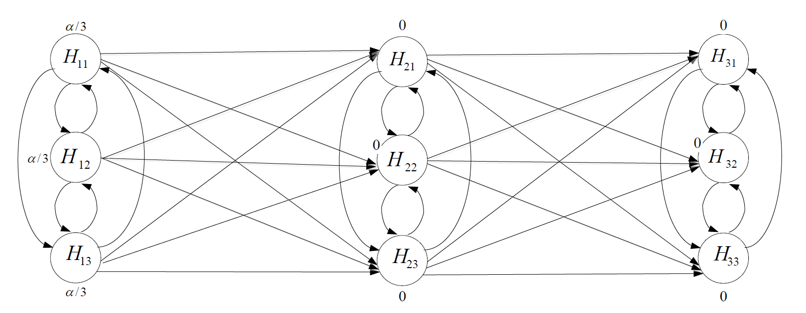
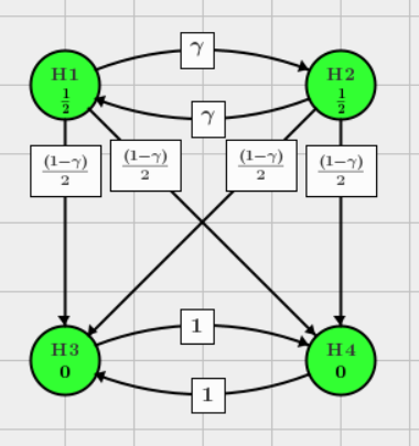
Figure - A intuitive example of Hypothesis-based graphical visualization of gatekeeping procedure with truncated Holm procedure with truncation parameter $\gamma$ as gatekeeper.

Basic notation

Suppose there are $N \ge 2$ hypotheses divided into $m \ge 2$ families, which are further grouped into $n$ layers, with $L_i=\left \{ F_{i1},F_{i2},...,F_{il_i} \right \}$ being the $i$-th ordered layer consisting of $l_i$ families of hypotheses, $i=1,...,n$ and $\sum_{i=1}^n l_i=m$.

Each family $F_{ij}$ within layer $L_i$ has $n_{ij} \ge 1$ null hypotheses, denoted as $F_{ij}=\left \{ H_{ij1},...,H_{ijn_{ij}} \right\}$ , for $j=1,..,l_i$, such that $\sum_{i=1}^n \sum_{j=1}^{l_i} n_{ij}=N$.

These families $F_{ij}$ of hypotheses are to be tested based on their respective p-value $P_{ijk},\ \ k=1,...,n_{ij}$, subject to controlling an overall measure of type I error at a pre-specified level $\alpha$.

Each of the true null p-value is assumed to be stochastically greater than or equal to the uniform distribution on $[0,1]$. That is, if $T_{ij}$ is the set of true null hypotheses in $F_{ij}$, then for any fixed $u \in [0,1]$, \[ \text{Pr}[P_{ijk} \le u \mid H_{ijk} \in T_{ij}] \le u, \] for any $i=1,...,n; \ \ j=1,...,l_i$ and $k=1,...,n_{ij}$.

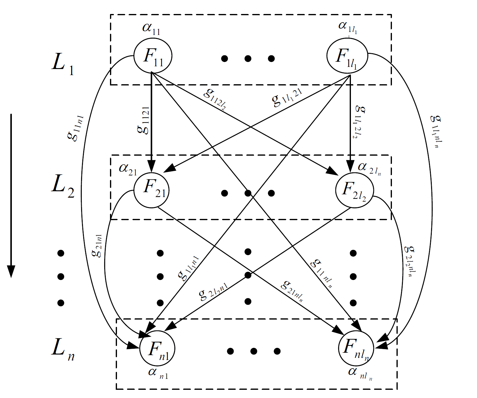
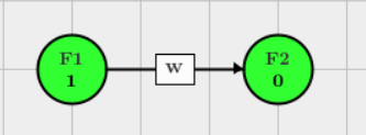
Figure - Graphical representation of general family-based graphical approach. Each vertex is associated with a family instead of a hypothesis, we term the graph as a family-based graph.

Global type I error rate control

The familywise error rate (FWER), which is the probability of incorrectly rejecting at least one true null hypothesis, is a commonly used notion of an overall measure of type I error when testing a single family of hypotheses.

Since we have multiple layers with any number of families within each layer, we consider this measure not locally for each family but globally. In other words, we deﬁne the overall FWER as the probability of incorrectly rejecting at least one true null hypothesis across all families of hypotheses for all layers.

"Layer" is an important concept in this paper! It represents the hierarchical structures over families instead of single hypothesis.

If it is bounded above by $\alpha$ regardless of which and how many null hypotheses within each family are true for any layer, then this overall FWER is said to be strongly controlled at $\alpha$.

Given the pre-specified $\alpha$, let $\alpha_i$ denote the initial critical values assigned to layer $L_i$ with $\sum_{i=1}^n \alpha_i \le \alpha$.

Remarks on error rate function introduced in Dmitrienko et al. (2008)

The error rate function was used to develop a simple stepwise approach for parallel gatekeeping strategies. In their discussion, the error rate function is required to be strictly less than $\alpha$ unless all of the hypotheses in one family are rejected, which is termed as separability condition.

Note that in applications, if the error rate function $e(\cdot)$ cannot be calculated easily, we often use one of its upper bounds $e^\ast(\cdot)$ to replace it.

The deﬁnition of the error rate function in this section we used is a a little bit more general. For this function, the separability condition is not required when choosing local procedures for our suggested family-based graphical approach.

In the family-based approach, each family is tested by its own local procedure, thus it is associated with a particular error rate function $e^\ast(\cdot)$.

Let $\alpha^{\ast}_{ij}$ denotes the local critical value for testing family $F_{ij}$ and $A_{ij}$ denote the set of accepted hypotheses in $F_{ij}$.

Based on $A_{ij}$, we can calculate $e^\ast(A_{ij})$ after testing $F_{ij}$ at level $\alpha^{\ast}_{ij}$ and then transfer the remaining amount of its local critical value $\alpha^{\ast}_{ij}-e^\ast(A_{ij})$ to their respective families in the subsequent layers according to the corresponding transition coefficients.

Testing procedures and alpha transition approach

The procedures start with testing $L_1$ to $L_n$ sequentially and within each layer $L_i$, families $F_{ij}$ are tested in any order using any local procedures based on their own (local) critical values.

The critical values used to locally test each family within the current layer is updated from its initially assigned value to one which incorporates certain portions of the critical values used in testing the families within the previous layers. This procedure stops testing when all families of the last layer $L_n$ are tested.

The distribution of the amount of critical values transferred among families can be pre-fixed by a transition coefficient set $G$ which is defined as follows.

Transition coefficient set G

Let $G=\left \{ g_{ijkl} \right \}$ denote a set of all transition coefficients $g_{ijkl}$ which satisfies the following conditions for any $i = 1,...,n$ and $j = 1,...,l_i$:

$$ \sum_{k=i+1}^n \sum_{l=1}^{l_k} g_{ijkl} \le 1; $$

and

$$ 0 \le g_{ijkl} \le 1; \ \ g_{ijkl}=0 \text{ if } i \ge k. $$

The $g_{ijkl}$ is defined as the proportion of the local critical value that can be transferred from family $F_{ij}$ within layer $L_i$ to family $F_{kl}$ within layer $L_k$. The above figure shows the graphical representation of the general family-based approach.

Algorithm

Algorithm 1 - Two layers with two families of hypotheses within each layer

Consider $m = 4$ families of hypotheses being divided into two layers $L_1=\left \{ F_{11},F_{12} \right \}, L_2=\left \{ F_{21},F_{22} \right \}$ based on their hierarchal relationships, with two families of hypotheses within each layer.

Graph for two layer family-based procedure with m=4.

Step $1$

Test family $F_{1j},j=1,2$ using any FWER controlling procedure at critical value $\alpha_{1j}$ and calculate $e^\ast(A_{1j})$.

Update the graph with \[ \begin{matrix} L_1 \to L_1 \setminus \left \{ F_{1j} \right \};\text{ for } k=1,2 \\\\ \text{let } \alpha_{2k} \to \alpha_{2k}+(\alpha_{1j}-e^{\ast}_{1j}(A_{1j}))g_{1j2k}; \end{matrix} \] and \[ g_{1l2k}= \left\{\begin{matrix} g_{1l2k}, & l \ne j \\\\ 0, & \text{otherwise.} \end{matrix}\right. \] if $L_1 \ne \emptyset$, go back to step $1$; otherwise, go to next step.

Step $2$

Test $F_{2k}, k = 1, 2$, using any FWER controlling procedure at level $\alpha_{2k}$ and update the graph: \[ L_2 \to L_2 \setminus \left \{ F_{2k} \right \}. \] If $L_2 \ne \emptyset$, go back to step $2$; otherwise stop.

步骤简述：
此算法从第一层$L_1$的假设检验族 family $F_{1j},j=1,2$ 开始执行；
一旦$F_{1j}$被检验，$F_{2k}$ 的检验水准将基于转移矩阵$G$和error rate function $e^{\ast}_{1j}(A_{1j})$更新，并且$G$的更新将删除所有的与$F_{1j}$相关的元素。
该算法的证明见原论文Appendix A.1。

Algorithm 2 - General multi-layer family-based graphical approach

The aforementioned two-layer four-family case demonstrates the inherent nature of sequential testing of the family-based graphical approach.

Now we generalize the graphical approach from two layers with two families of hypotheses in each layer to any $n$ layers with arbitrary number of families of hypotheses within each layer.

The general multi-layer family-based graphical approach is deﬁned through the following algorithm:

Step $i \ \ (1 \le i \le n-1 )$

Test family $F_{ij},j=1,2,...,l_i$ using any FWER controlling procedure at critical value $\alpha_{ij}$ and calculate $e_{ij}^\ast(A_{ij})$.

Update the graph with \[ \begin{matrix} L_i \to L_i \setminus \left \{ F_{ij} \right \};\text{ for } k=i+1,...,n; l=1,...,l_k \\\\ \text{let } \alpha_{kl} \to \alpha_{kl}+(\alpha_{ij}-e_{ij}^{\ast}(A_{ij}))\times g_{ijkl}; \end{matrix} \] and \[ g_{iskl}= \left\{\begin{matrix} g_{iskl}, & s \ne j \\\\ 0, & \text{otherwise.} \end{matrix}\right. \] if $L_i \ne \emptyset$, go back to step $i$; otherwise, go to next step.

Step $n$

Test $L_n = \left \{ F_{n1},...,F_{nl_n} \right \}$, using any FWER controlling procedure at level $\alpha_{nj}$ to test $F_{nj}$ and update the graph: \[ L_n \to L_n \setminus \left \{ F_{nj} \right \}. \] If $L_n \ne \emptyset$, go back to step $n$; otherwise stop.

简单案例：
考虑一个有$n$层$L_1,...,L_n$，并且每层$L_{i}$只有一个假设检验族$F_{i1}$的多重检验。
在多层family-based graphical approach下，$F_{i1}$ 的初始检验水准是$\alpha$，如果$i=1$；其余family分到的检验水准都是0。此时transition coefficient为$g_{i1k1}=1$，如果$1 \le i \le n-1, \ \ k=i+1$ 。其他情况下$g_{i1k1}=0$。
该算法的证明见原论文Appendix A.2。

对于上述算法，有以下几点额外的考量：

如果每个family都使用了能控制住FWER的local procedure，并且这些procedure都能满足separability condition (i.e. 每个local procedure的error rate function都严格小于$\alpha$)，那么这个算法等价于parallel gatekeeping中的general multistage gatekeeping procedure (Dmitrienko et al.(2008))。这个非常重要，表示truncated step-wise的传统检验步骤可以被图形化；
如果每个family都使用了能控制住FWER的local procedure，并且这些procedure的error rate function的上确界为$e^{\ast}(I)=\alpha, \text{ for any } I \ne \emptyset$，那么这个算法等价于特定的serial gatekeeping，比如传统Holm，fixed sequence procedure等；
如果每个family都只有1个假设检验，其等价于fixed sequence procedure；
如果一个family内，null p-values之间的相关性已知，那么对于local procedures我们有更多选择，比如传统或者truncated Hochberg.

Example 1

Consider the Type II diabetes clinical trial example in Dmitrienko et al. (2007).

The trial compares three doses of an experimental drug (Doses L, M and H) versus placebo (Plac) with respect to one primary endpoint (P: Haemoglobin A1c), and two secondary endpoints (S1: Fasting serum glucose; S2: HDL cholesterol).

The three endpoints will be examined at each of the three doses, so a total of nine null hypotheses will be formulated and grouped into three families, $F_1$, $F_2$ and $F_3$.

Family $F_1$ consists of three dose-placebo comparisons corresponding to the primary endpoint

H vs Plac ($H_{11}$)
M vs Plac ($H_{12}$)
L vs Plac ($H_{13}$)

Similarly, family $F_2$ and $F_3$ consists of three dose-placebo comparisons corresponding to the secondary endpoint and family F3 consists of three dose-placebo comparisons corresponding to the secondary endpoint.

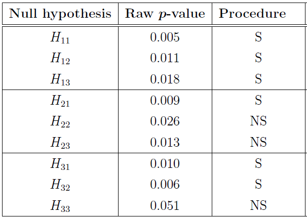
The overall Type I error rate is pre-speciﬁed at $\alpha=0.05$ and the raw p-values for the nine null hypotheses are given in the following table.

In this example, we assume that the primary endpoint P is more important than the secondary endpoints S1 and S2, thus F1 is always tested before testing F2 and F3.

Suppose that the secondary endpoints S1 and S2 are equally important, thus F2 and F3 are grouped into the same layer; the dose-placebo comparisons within each family are ordered a priori (H vs. Plac through L vs. Plac).

We choose the conventional ﬁxed sequence procedure as local procedure for each family and the initial allocation of critical values for $F_1$, $F_2$ and $F_3$ are 0.04, 0.005, and 0.005, respectively. Once $F_1$ is tested and all of its hypotheses are rejected, its critical value is equally allocated to $F_2$ and $F_3$.

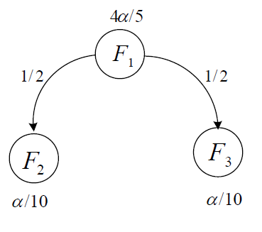
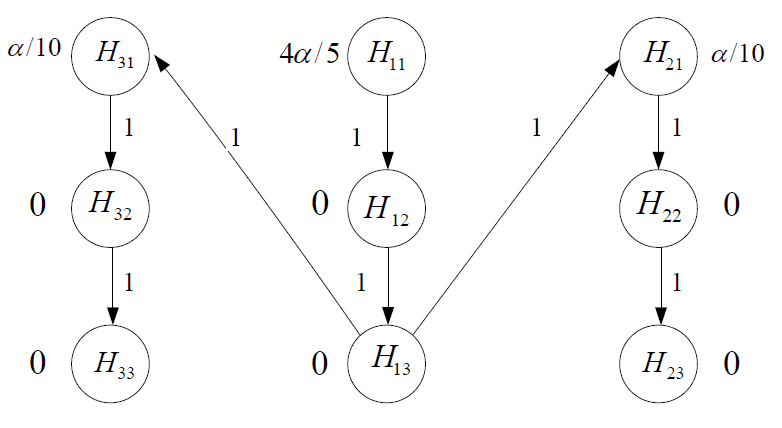
The above figure visualizes this gatekeeping strategy. We start testing $F_1$ at level 0.04; all of three hypotheses in $F_1$ are rejected using the conventional ﬁxed sequence procedure.

Then, all of its local critical value 0.04 is equally assigned to $F_2$ and $F_3$ and the updated critical values for $F_2$ and $F_3$ become $0.005 + 0.02 = 0.025$. We continue to test $F_2$ and $F_3$ at level 0.025 in any order using the conventional ﬁxed sequence procedure; the resulting rejected hypotheses are $H_{21}, H_{31}$ and $H_{32}$.

Finally, the testing results of Procedure are summarized in the above table. In addition, a figure below provides a graphical visualization for Procedure by using the hypothesis-based graphical approach.

Example 2

Consider an example as below

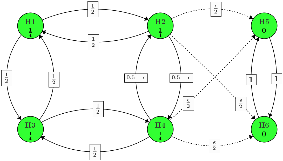
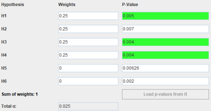
In hypothesis-based graphical approach, the initial weights for hypotheses $H_1,H_2,H_3,H_4$ are $\frac{1}{4}\alpha=\frac{1}{4} \times 0.025=0.00625$ respectively. The $\epsilon$ denotes the infinitesimally small weight for significance shifting between families.

Suppose the raw p-value for these 6 hypotheses are

In the environment of R, the $\epsilon$ is approximated as 0.00001. The code of generating the gMCP graph is

m <- rbind(H1=c(0, 0.5, 0.5, 0, 0, 0),
           H2=c(0.5, 0, 0, "0.5-\\epsilon", "\\epsilon/2", "\\epsilon/2"),
           H3=c(0.5, 0, 0, 0.5, 0, 0),
           H4=c(0, "0.5-\\epsilon", 0.5, 0, "\\epsilon/2", "\\epsilon/2"),
           H5=c(0, 0, 0, 0, 0, 1),
           H6=c(0, 0, 0, 0, 1, 0))
weights <- c(0.25, 0.25, 0.25, 0.25, 0, 0)
graph1 <- new("graphMCP", m=m, weights=weights)
pvalues <- c(0.005, 0.007, 0.004, 0.004, 0.00626, 0.002)
gMCP(graph1, pvalues, test="Bonferroni", alpha=0.025,verbose = TRUE, eps = 0.00001)

# Import to GUI
graphGUI(graph1,pvalues=pvalues)

注意：gMCP()在RStudio环境中极易崩溃，需用原生R来运行

We can break down the MTP into steps as

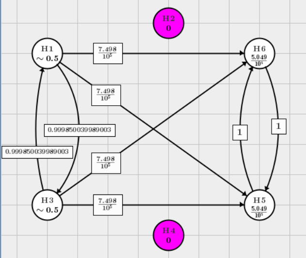
Reject $H_1$ and pass its level to $H_2$ and $H_3$
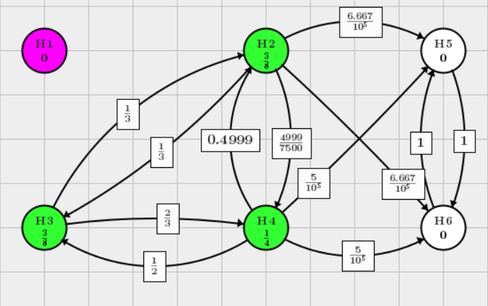
Reject $H_3$, note that $\frac{7.5}{10^5} \approx \frac{3}{4}\alpha$ using the Algorithm 1 in Bretz et al.(2009) to update the weight.

In this graph, $j=3, l=4, k=5$, the graph update algorithm is

$$ g_{lk} \leftarrow \frac{g_{lk}+g_{lj}g_{jk}}{1-g_{lj}g_{jl}}=\frac{\epsilon/2+1/2 \times 0}{1-1/2 \times 2/3}=\frac{3 \alpha}{4}. $$

其余权重更新具体数值可以根据这个公式计算

That is

This graph is updated to, and we can continuously reject $H_2$
Reject $H_4$
Finally both of $H_5$ and $H_6$ can be rejected.

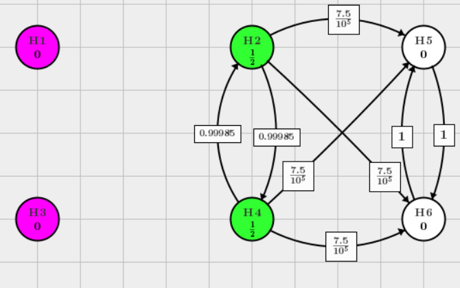
Could it be re-written as family-based graph approach?

Suppose $F_1=\left \{ H_1,H_3,H_2,H_4 \right \} \subset L_1$, $F_2=\left \{ H_5,H_6 \right \} \subset L_2$.

It is obvious that $F_1$ is more important that $F_2$. Consider a case that all the hypotheses in $F_1$ are not significant, e.g.

1
2
3

# Suppose H1 and H3 are not significant!
pvalues2 <- c(0.08, 0.007, 0.08, 0.004, 0.00626, 0.002)
graphGUI(graph1,pvalues=pvalues2)

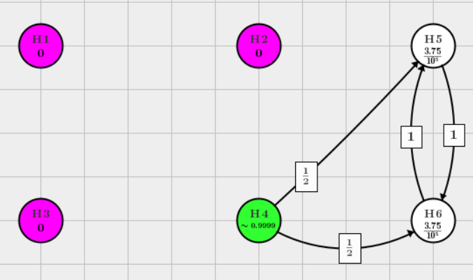
After rejecting $H_2, H_4$ in $F_1$, the graph turns into the following one

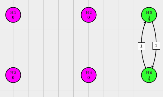
$F_2$ can not be tested unless the hypotheses in $F_1$ is significant.

由此，我们可以看出该检验的层次结构，$F_1$ 与 $F_2$具有同等重要性，而$F_3$的检验需要基于$F_1$与$F_2$ 的检验结果。

The family-based graph looks like

Example 3 - Truncated Holm

Consider the 4 hypotheses truncated holm MTP (parallel gatekeeping) in hypothesis-based graph approach and the prespecified significance level is $\alpha=0.05$. The detailed algorithm of truncated holm is described in Dmitrienko et al. (2008).

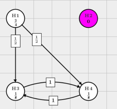
Let $F_1=\left \{ H_1,H_2 \right \}$ and $F_2=\left \{ H_3,H_4 \right \}$.

If $H_2$ is rejected, $j=2, l=1, k=3$, the graph update algorithm based on the removal of $H_2$ is

$$ g_{13} \leftarrow \frac{g_{13}+g_{31}g_{23}}{1-g_{21}g_{12}}=\frac{1-\gamma + \gamma -\gamma^2}{2(1-\gamma^2)}=1/2. $$

Similarly, $g_{14}=1/2$:

In family-based graphical approach,

where weight $w$ in the graph is calculated based on the error rate function \[ w=\left\{\begin{matrix} 1-[\gamma + \frac{1-\gamma}{n} \mid A_1 \mid ] & ,A_1 \ne \emptyset \\\\ 1 & ,A_1 = \emptyset \end{matrix}\right. \] Note that $\mid A_1 \mid$ is the number of hypotheses accepted in $F_1$ and $n$ is the number of hypotheses in $F_2$.

Firstly, test hypotheses in $F_1$ using truncated Holm:

If all hypotheses in $F_1$ are tested and rejected using truncated Holm at initial $\alpha_1=\alpha=0.05$, the $w=1$ since $A_1 = \emptyset$. Therefore, $F_2$ will be tested on level $\alpha_2=\alpha_1-0=\alpha$;
If only one hypothesis in $F_1$ is tested and rejected at initial $\alpha_1=\alpha=0.05$, the $w=\frac{1}{2}-\frac{1}{2}\gamma$ since $A_1 \ne \emptyset$. That is, $F_2$ will be tested on level $\alpha_2=\alpha_1-e^{\ast}(A_1)=\alpha-[\gamma+\frac{1-\gamma}{2}]\alpha=[\frac{1}{2}-\frac{1}{2}\gamma]\alpha$;
If all hypotheses in $F_1$ are tested and accepted using truncated Holm at initial $\alpha_1=\alpha=0.05$, the $w=0$. Therefore, $F_2$ will not be tested.

Reference

Bretz, Frank & Maurer, Willi & Brannath, Werner & Posch, Martin. (2009). A graphic approach to sequentially rejective multiple test procedures. Statistics in medicine. 28. 586-604. 10.1002/sim.3495.

Dmitrienko, Alex & Tamhane, Ajit & Wiens, Brian. (2008). General Multistage Gatekeeping Procedures. Biometrical journal. Biometrische Zeitschrift. 50. 667-77. 10.1002/bimj.200710464.

Qiu, Zhiying & Li, Yu & Guo, Wenge. (2018). A Family-based Graphical Approach for Testing Hierarchically Ordered Families of Hypotheses. 10.13140/RG.2.2.23109.29929.