Linear Model in SAS (1) - Type I~IV SS and Contrast/Estimate Statement
PROC REG can compute two types of sums of squares associated with the estimated coefficients in the model. These are referred to as Type I and Type II sums of squares and are computed by specifying SS1 or SS2, or both, as MODEL statement options.
1 | proc reg; |
In particular, the concepts of partitioning sums of squares, complete and reduced models, and reduction notation are useful in understanding the different types of sums of squares.
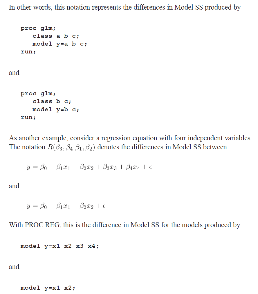
Reduction Notation
Partitioning the Sums of Squares
The following formula
\[ \text{TOTAL SS = MODEL SS + ERROR SS} \]
is equivalent to
\[ \sum (y-\bar{y})^2 = \sum (\hat{y}-\bar{y})^2 + \sum (y-\hat{y})^2. \]
Based on the common notations for interpreting linear models using matrix theory, the residual or error sum of squares is
\[ \text{ERROR SS} = Y'(I-X(X'X)^{-1}X')Y=Y'Y-\hat{\beta}X'Y. \]
The error mean square
\[ s^2=\text{MSE}=\frac{\text{ERROR SS}}{n-m-1} \]
is an unbiased estimate of \(\sigma^2\), the variance of \(\epsilon_i\).
PROC REG and PROC GLM compute several sums of squares. Each sum of squares can be expressed as the difference between the regression sums of squares for two models, which are called complete and reduced models. This approach relates a given sum of squares to the comparison of two regression models.
Denote by MODEL SS1 the MODEL SS for a regression with \(m = 5\) variables:
\[ y=\beta_0 + \sum_{i=1}^{5}\beta_i x_i + \epsilon, \]
and by MODEL SS2 the MODEL SS for a reduced model not containing \(x_4\) and \(x_5\):
\[ y=\beta_0 + \sum_{i=1}^{3}\beta_i x_i + \epsilon, \]
Reduction in sum of squares notation can be used to represent the difference between regression sums of squares for the two models.
For example,
\[ \text{R}(\beta_4,\beta_5 \mid \beta_0,\beta_1,\beta_2,\beta_3)=\text{MODEL SS1 - MODEL SS2} \]
The difference, or reduction in error, \(\text{R}(\beta_4,\beta_5 \mid \beta_0,\beta_1,\beta_2,\beta_3)\) indicates the increase in regression sums of squares due to the addition of \(\beta_4\) and \(\beta_5\) to the reduced model.
The expression \(\text{R}(\beta_4,\beta_5 \mid \beta_0,\beta_1,\beta_2,\beta_3)\) is also commonly referred to as
- the sum of squares due to \(\beta_4\) and \(\beta_5\) (or \(x_4\) and \(x_5\)) adjusted for \(\beta_0,\beta_1,\beta_2,\beta_3\) (or the intercept and \(x_1,x_2,x_3\));
- the sum of squares due to fitting \(x_4\) and \(x_5\) after fitting the intercept and \(x_1,x_2,x_3\);
- the effects of \(x_4\) and \(x_5\) above and beyond, or partial of, the effects of the intercept and \(x_1,x_2,x_3\).
From SAS online doc v8,
Type I SS
The Type I SS are commonly called sequential sums of squares. They represent a partitioning of the MODEL SS into component sums of squares due to adding each variable sequentially to the model in the order prescribed by the MODEL statement.
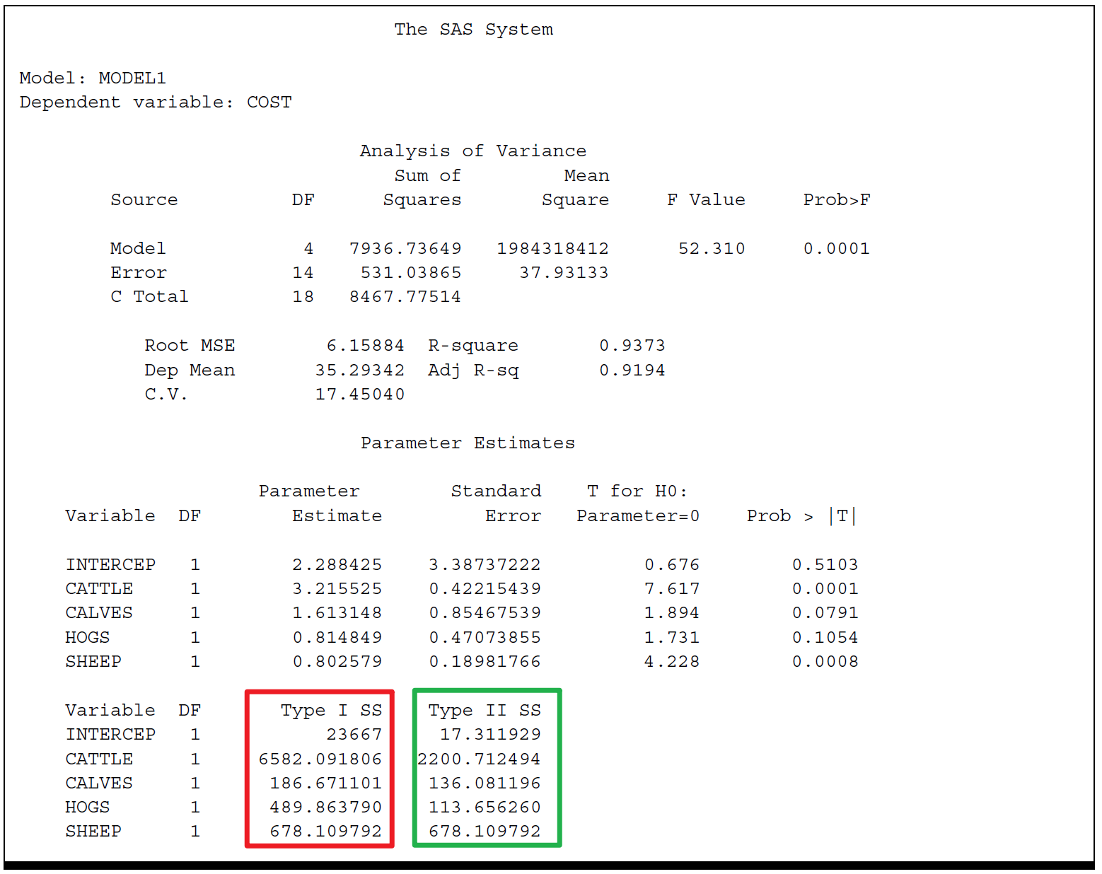
The Type I SS for the INTERCEP is simply \(n\bar{y}^2\) . It is called the correction for the mean. It's \(23667\).
Type I SS for CATTLE (\(6582.09181\)) is the MODEL SS for a regression equation that contains only CATTLE.
The Type I SS for CALVES (\(186.67110\)) is the increase in MODEL SS due to adding CALVES to the model that already contains CATTLE.
In general, the Type I SS for a particular variable is the sum of squares due to adding that variable to a model that already contains all the variables that preceded the particular variable in the MODEL statement.
Note that the following equation illustrates the sequential partitioning of the MODEL SS [a] into the Type I components that correspond to the variables in the model. \[ \text{MODEL Sum of Squares} = 7936.7= 6582.1 + 186.7 + 489.9 + 678.1 \]
Type II SS
The Type II SS are commonly called the partial sums of squares. For a given variable, the Type II SS is equivalent to the Type I SS for that variable if it were the last variable in the MODEL statement.
Type II SS for a particular variable is the increase in MODEL SS due to adding the variable to a model that already contains all the other variables in the MODEL statement.
The Type II SS, therefore, do not depend on the order in which the independent variables are listed in the MODEL statement. Furthermore, they do not yield a partitioning of the MODEL SS unless the independent variables are uncorrelated.
Type I/II SS
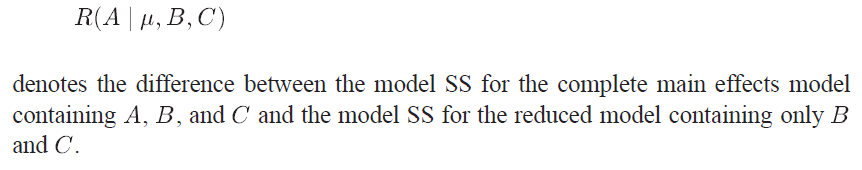
The Type I SS and Type II SS are shown in the table below in reduction notation
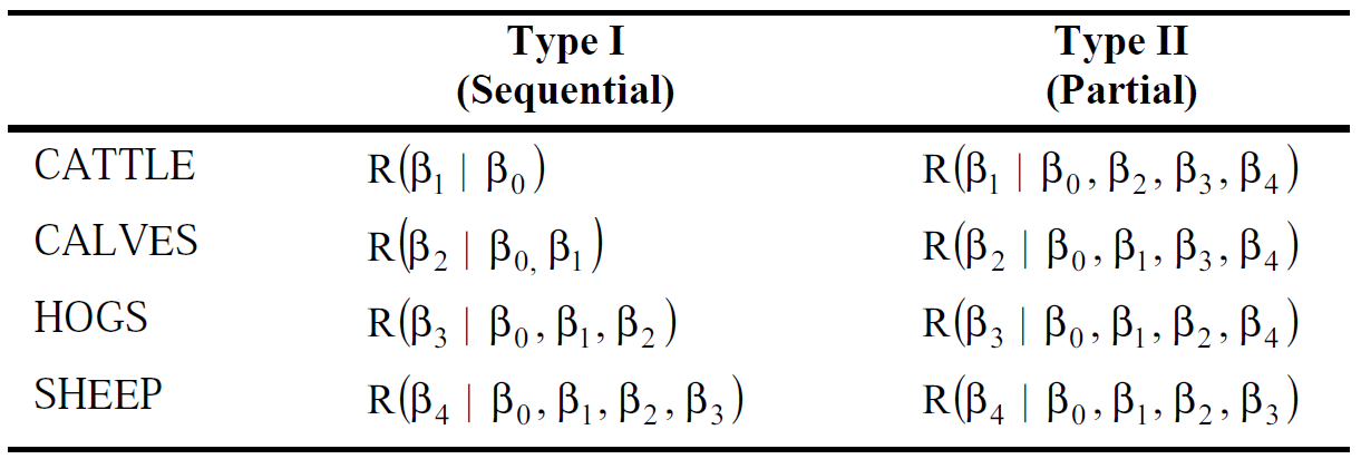
上表中对于第一行CATTLE,Type I SS表示往只有截距的模型中加入变量\(x_1\)后,两个模型MODEL SS之间的差异;
对于Type II SS,表示往有截距、\(x_2 \sim x_4\)的模型中加入变量\(x_1\)后,两个模型MODEL SS之间的差异;
Reduction notation给我们用F-test (基于SS构建)去比较complete model和reduced model提供了便利。
Model comparison
Degree of freedom
自由度 (DF) 是数据提供的信息量,您可以使用这些信息来估计未知总体参数的值并计算这些估计值的变异性。自由度值由样本中的观测值个数和模型中的参数个数确定。
换句话说,自由度是衡量你有多少数据的一种方法。例如,有\(N\)个观察值,就有\(N\)个自由度。但是如果通过减去平均值并除以标准差来 "标准化 "你的数据,你就会失去2个自由度。
一种思考方式是,如果你告诉我任何\(N-2\)个数据点,加上平均值和标准差,我可以计算出缺失的那2个数据点。即,只有\(N-2\)个数据点是 "自由 "的。
F-test with different SS
对于一个特定变量(2水平)来说,它的SS只有1个自由度,此时它的SS即为Mean squares,因为MS=SS/DF.
(1)
比如Type I F-test,对于CALVES为 \[ F=\frac{\text{Type I SS}}{MSE}=\frac{186.7}{37.9}=4.92 \] 这个F值用来检验包含CATTLE和CALVES的complete model,是否显著优于仅包含CATTLE的reduced model。因为来源于Type I SS,它本身就包含了一种模型比对的含义(difference in SS)。
(2)
对于Type II SS,CALVES的F统计量为 \[ F=\frac{\text{Type II SS}}{MSE}=\frac{136.1}{37.9}=3.59 \] 这个F值用来检验包含CATTLE,CALVES,HOGS和SHEEP的complete model,是否显著优于仅包含CATTLE,HOGS和SHEEP的reduced model。因为来源于Type I SS,它本身就包含了一种模型比对的含义(difference in SS)。
Type I/II SS for F-test & T-test
现在应该指出,Type II F-检验完全等同于参数的 t-检验,因为它们比较的是相同的complete model和reduced model。事实上,一个给定变量的Type II F-统计量等于同一变量的 t-统计量的平方。
在大多数应用中,对单个参数(single parameter)的检验是基于Type II SS的,这相当于参数估计的 t检验。然而,如果需要对单个回归系数(individual coefficients)进行特定的检验排序,例如在多项式模型中,Type I SS是有用的。
Type III/IV SS
see [b]
Contrast in PROC GLM
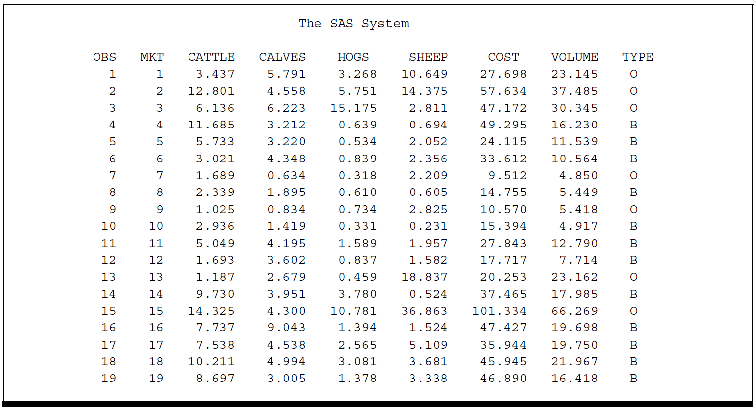
Model fit1
2
3proc glm;
model cost=cattle calves hogs sheep;
run;
Results appear in the following output
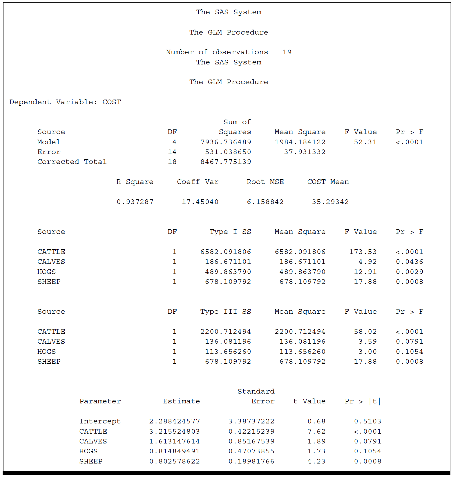
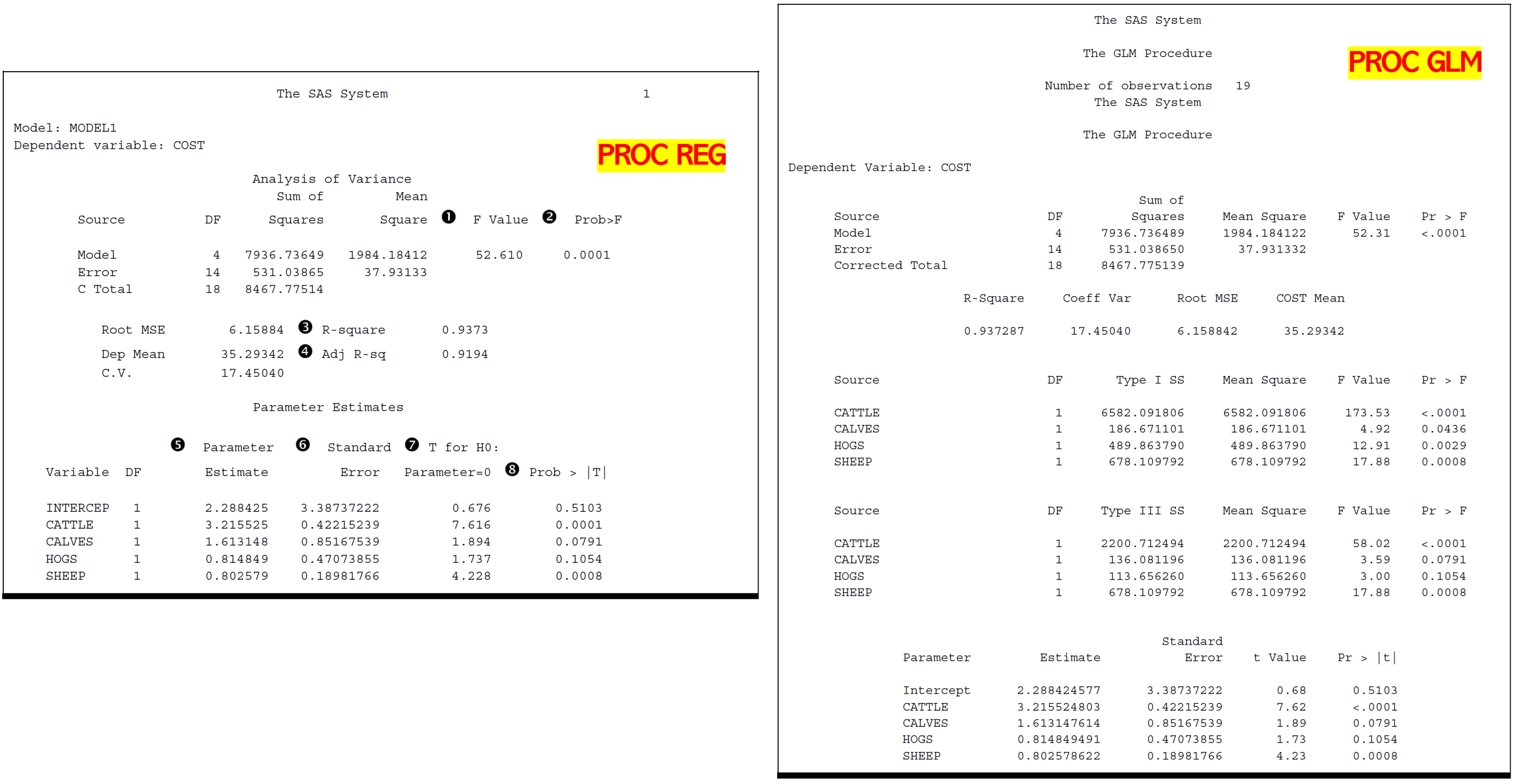
Compare it with the previous output, we find the same partition of sums of squares, with slightly different labels, the same R-square, Root MSE, F-test for the Model, and other statistics. In addition, we find the same parameter estimates.
Type I ~ IV SS [b]
The Type I sums of squares are the same from PROC GLM and PROC REG.
We also see that the Type III sums of squares from GLM are the same as the Type II sums of squares from PROC REG. In fact, there are also Types II and IV sums of squares available from PROC GLM whose values would be the same as the Type II sums of squares from PROC REG.
In general, Types II, III, and IV sums of squares are identical for regression models, but differ for some ANOVA models.
CONTRAST Statement to Test Hypotheses about Regression Parameters
Recap
- Test \(H_0: \beta_1=\beta_2=\beta_3=\beta_4=0\) using test statistic \(F=\text{MS MODEL}/ \text{MS ERROR}\);
- Test individual parameter like \(H_0: \beta_2=0\) using an F-statistic based on either the Type I or the Type II sum of squares. [注:可用reduced notation帮助理解]
*Using Contrast statement
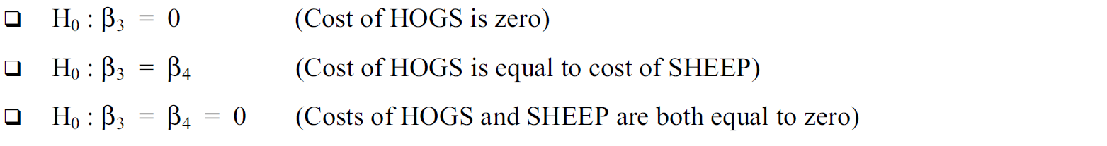
We want to test the following hypotheses using CONTRAST statement:
The basic syntax of the CONTRAST statement is1
2
3
4* effect values refers to coefficients of a linear combination of parameters;
* label simply refers to a character string to identify the results in the PROC GLM output;
contrast 'label' effect values;
For our regression example, a hypothesis about a linear combination of parameters would have the form \[ H_0: a_0 \beta_0+a_1 \beta_1+a_2 \beta_2 +a_3 \beta_3+a_4 \beta_4= 0 \] where \(a_0,a_1,a_2,a_3,a_4\) are numbers.
其实这里等价于subset of hypotheses test里的 \(\mathbf{L} \mathbf{ \beta}=0\),其中\(\mathbf{L}=[a_0,a_1,a_2,a_3,a_4]\), \(\mathbf{\beta}=[\beta_0,\beta_1,\beta_2,\beta_3,\beta_4]^T\)
This hypothesis would be indicated in a CONTRAST statement as1
contrast 'label' intercept a0 cattle a1 calves a2 hogs a3 sheep a4;
For the hypotheses testing we are interested in,
\(H_0: \beta_3=0\): the linear combination in this hypothesis is simply \(\beta_3 \times 1\), so \(\mathbf{L}=[a_0=0,a_1=0,a_2=0,a_3=1,a_4=0]\). Therefore, we could use the CONTRAST statement
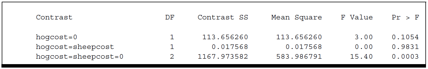
contrast 'hogcost=0' intercept 0 cattle 0 calves 0 hogs 1 sheep 0;事实上,我们仅需要指定non-zero的参数即可,上面指令可简化为
contrast 'hogcost=0' hogs 1;\(H_0: \beta_3=\beta_4 \text{ which is equivalent to } \beta_3-\beta_4=0\): the linear combination in this hypothesis is simply \(\mathbf{L}=[a_0=0,a_1=0,a_2=0,a_3=1,a_4=-1]\). Therefore, we could use the CONTRAST statement
contrast 'hogcost=sheepcost' hogs 1 sheep -1;\(H_0: \beta_3=\beta_4=0 \text{ which is equivalent to } \beta_3=0 \text{ and } \beta_4=0\): the linear combination in this hypothesis should be written as two combinations
contrast 'hogcost=sheepcost=0' hogs 1, sheep 1;
Now run the statements1
2
3
4
5
6proc glm;
model cost=cattle calves hogs sheep;
contrast ‘hogcost=0’ hogs 1;
contrast ‘hogcost=sheepcost’ hogs 1 sheep -1;
contrast ‘hogcost=sheepcost=0’ hogs 1, sheep 1;
run;
Results of the CONTRAST statements appear in the following output
Estimate in PROC GLM
Sometimes it is more meaningful to estimate the linear combinations. We can do this with the ESTIMATE statement in PROC GLM.
The ESTIMATE statement is used in essentially the same way as the CONTRAST statement.
But instead of F-tests for linear combinations, we get estimates of them along with standard errors.
However, the ESTIMATE statement can estimate only one linear combination at a time, whereas the CONTRAST statement could be used to test two or more linear combinations simultaneously.
Consider the first two linear combinations we tested, namely \(\beta_3\) and \(\beta_3-\beta_4\). We can estimate these linear combinations by using the ESTIMATE statements1
2estimate 'hogcost=0' hogs 1;
estimate 'hogcost=sheepcost' hogs 1 sheep -1;
Result
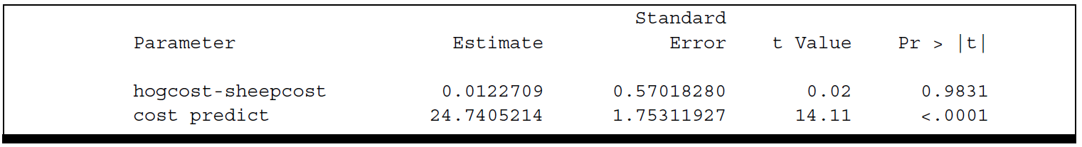
The advantage of the ESTIMATE statement is that it gives us estimates of the linear combinations and standard errors in addition to the tests of significance.
PROC REG v.s. PROC GLM
PROC GLM is very similar to that of PROC REG for fitting linear regression models. Beyond the basic applications the two procedures become more specialized in their capabilities.
PROC REG :
- has greater regression diagnostic and graphic features.
But PROC GLM :
- has the ability to create "dummy" variables. This makes
PROC GLMsuited for- analysis of variance,
- analysis of covariance, and
- certain mixed-model applications.
With regards to Type I/II SS
PROC REG does not compute F-values for the Type I and Type II sums of squares, nor does it compute the corresponding significance probabilities.
However, we can use PROC GLM to make the same computations discussed in this chapter.
There are several other distinctions between the capabilities of PROC REG and PROC GLM. Not all analyses using PROC REG can be easily performed by PROC GLM.