Let's have a look at some algebra of linear model in SAS. We'll skip the simple knowledge points commonly found in textbooks in this post.

General Notations

The REG and GLM procedures implement a multiple linear regression analysis according to the model \[ y=\beta_0+\sum_{i=1}^m \beta_i x_i + \epsilon, \] where \(x_i\) are independent and \(\epsilon\) is the error term.

The model in the matrix notation is \[ \mathbf{Y=X \beta+\epsilon}, \] which is

\(n\) is the #observations and \(m\) is the #variables.

We have unique solution \(\hat{\beta}=(X'X)^{-1}X'Y\) with assumption that \(X'X\) has full rank, and the \((X'X)^{-1}\) is often denoted by

The \(\mathbf{C}\) matrix provides the variances and covariances of the regression parameter estimates \[ V(\hat{\beta})=\sigma^2 \mathbf{C}, \] where \(\sigma^2=V(\epsilon_i)\).

Partitioning the Sums of Squares

Recall

TOTAL SS = MODEL SS + ERROR SS

A basic identity results from least squares, specifically, \[ \sum (Y-\bar{Y})^2=\sum (\hat{Y}-\bar{Y})^2+\sum (Y-\hat{Y})^2 \] The total sum of squared deviations from the mean can be partitioned into two parts:

• the sum of squared deviations from the regression line to the overall mean

  \(\sum (\hat{Y}-\bar{Y})^2\);

• the sum of squared deviations from the observed \(y\) values to the regression line

  \(\sum (Y-\hat{Y})^2\).

In matrix notation, the residual or error sum of squares is \[ \text{ERROR SS}=\mathbf{Y'(I-X(X'X)^{-1}X')Y=Y'Y-\hat{\beta}X'Y} \] The error mean square (MSE) \[ s^2=\frac{\text{ERROR SS}}{n-m-1}=\mathbb{E}[\sigma^2] \] which is an unbiased estimate of \(\sigma^2\), the variance of \(\epsilon_i\).

PROC REG and PROC GLM compute several sums of squares.

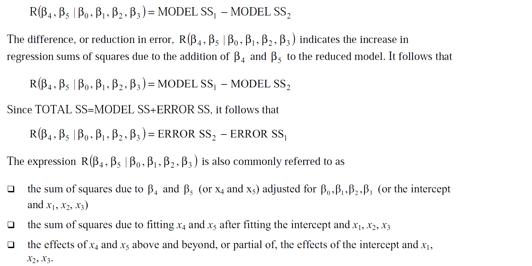
Each sum of squares can be expressed as the difference between the regression sums of squares for two models, which are called complete and reduced models.

This approach relates a given sum of squares to the comparison of two regression models.

Reduction in sum of squares

Reduction in sum of squares notation can be used to represent the difference between regression sums of squares for the two models.

Hypothesis Tests and Confidence Intervals

Inferences about model parameters are highly dependent on the other parameters in the model under consideration.

Therefore, in hypothesis testing it is important to emphasize the parameters for which inferences have been adjusted.

Statistical inferences can also be made in terms of linear functions of the parameters in the form \[ H_0: \sum_{j=0}^m l_j \beta_j =0. \] Note that \(l_j\) are constants chosen to correspond to a specified hypothesis. Such functions are estimated by the corresponding linear function (之所以说是“estimated”，是因为这里的式子可以看做是\(\beta_j\)的一个线性组合) \[ \mathbf{L\hat{\beta}}=\sum_{j=0}^m l_j \hat{\beta_j} \] of the least-squares estimates (OLE) \(\hat{\beta}\). The variance of \(\mathbf{L\hat{\beta}}\) is \[ V(\mathbf{L\hat{\beta}})=(\mathbf{L(X'X)^{-1}L'})\sigma^2. \] 对于假设检验\(H_0: \mathbf{L\beta}=0\)，我们可以用t test或者F test去检验。分母通常为MSE (estimate of \(\sigma^2\))。从\(V(\mathbf{L\hat{\beta}})\)可以看到，这个estimated function的方差取决于整个模型的统计量，假设的检验是在所有模型参数存在的情况下进行的。这些检验可以被概括为对几个线性函数的同时检验。同时，我们可以构建对应于检验的置信区间。

Three common types of statistical inference（推断）

1 - Test all slope parameters are 0

即比较complete model与minimal model （null model仅包含截距）。

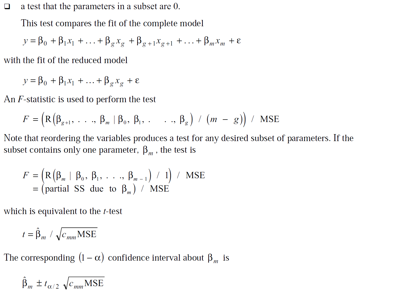
2 - Test the parameters in a subset are 0

前面的post有很多对subset检验的叙述。

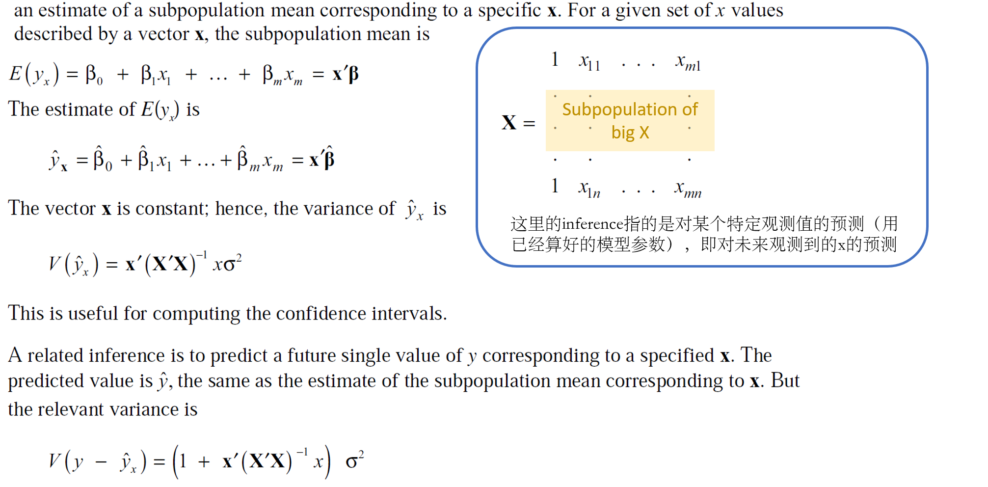
3 - Prediction on future X

Using the Generalized Inverse

这个章节要解决什么问题？

答：很多场合下（比如PROC GLM建模时候），\(X'X\)是不满秩的（of full rank），意思是这个矩阵中有些行可以表示为其他行的线性组合，所以这种不满秩的\(X'X\)没有唯一的逆（unique inverse）。对于这种不满秩的场景，PROC GLM与PROC REG都会去计算一个generalized inverse (广义逆)，\((X'X)^-\)，并用它来计算回归参数\(\mathbf{b}=\mathbf{(X'X)^-X'Y}\)。

参考博文 Linear Model in SAS (2.1) - The Design Matrix Is Of Less Than Full Rank !

Generalized inverse of a matrix

A generalized inverse of a matrix \(\mathbf{A}\) is any matrix \(\mathbf{G}\) such that \(\mathbf{AGA=A}\). Note that this also identifies the inverse of a full-rank matrix. There is an infinite number of generalized inverses.

If \(X'X\) is not of full rank, different generalized inverses lead to different solutions to the normal equations that will have different expected values (因为存在无数个广义逆).

The normal equation is a closed-form solution used to find the value of parameters that minimizes the cost function.

That is, \(\mathbb{E}[\mathbf{b}]=\mathbf{(X'X)^-X'X\beta}\) depends on the particular generalized inverse used to obtain \(\mathbf{b}\). (即，模型参数的求解取决于特定的广义逆，进而引发思考，模型推断过程中，除了回归参数，还有什么计算需要用到广义逆？见下文)

Fortunately, not all computations in regression analysis depend on the particular solution obtained.

• For example, the error sum of squares has the same value for all choices of \(\mathbf{(X'X)^-}\) and is given by \(\text{SSE}=\mathbf{Y'(I-X(X'X)^-X')Y=Y'Y-\hat{\beta}X'Y}\). Hence, the model sum of squares also does not depend on the particular generalized inverse obtained. （即，error sum of squares对于不同的广义逆，都有相同的值，所以SSE不依赖特定的广义逆。同理，MODEL SS也不依赖于特定的广义逆）

但是在SAS计算过程中，广义逆作为中间步骤是需要计算出来的。

Consider, for example, an \(\mathbf{X'X}\) matrix of rank \(k\) that can be partitioned as

where \(\mathbf{A_{11}}\) is \(k \times k\) and of rank \(k\).

Then \(\mathbf{A_{11}^{-1}}\) exists（因为这个矩阵满秩，所以可逆）, and a generalized inverse of \(\mathbf{X'X}\) is

where each \(\phi_{ij}\) is a matrix of zeros of the same dimensions as \(\mathbf{A_{ij}}\). （可根据如下定理）

如上所示，这种获得广义逆的方法可以通过将一个奇异阵（singular matrix，行列式为0的矩阵，奇异阵都是可逆的）分割成几组矩阵来无限扩展。这种分割方式是无穷多的，所以广义逆也是无穷多的。

其中，normal equation \(\mathbf{b}=\mathbf{(X'X)^-XY}\)的解，在广义逆矩阵\(\mathbf{(X'X)^-}\)为0的行对应的位置上有0值。这个解会在PROC GLM或者PROC REG的输出中汇报。

这一句英文原文：Note that the resulting solution to the normal equations, \(\mathbf{b}=\mathbf{(X'X)^-XY}\) has zeros in the positions corresponding to the rows filled with zeros in \(\mathbf{(X'X)^-}\) .

注意！这个解是对回归参数 \(\mathbf{\beta}\) 的有偏估计！

再注意！由于 \(\mathbf{b}\) 不唯一（因为广义逆不唯一），所以 \(\mathbf{b}\) 的函数 \(\mathbf{Lb}\)，以及这个函数的方差\(\text{Var}[\mathbf{Lb}]\)也是不唯一的！

Estimable Functions

However, there is a class of linear functions called estimable functions, and they have the following properties：

1. The linear function \(\mathbf{Lb}\) and its variance are invariant through all possible generalized inverses. In other words, \(\mathbf{Lb}\) and \(\text{Var}[\mathbf{Lb}]\) are unique

2. The linear function \(\mathbf{Lb}\) is an unbiased estimate of \(\mathbf{L\beta}\)

   结合上面两条性质 （1）与（2），也就是说，可以找到回归参数的函数的无偏估计，这是非常振奋人心的！因为这也意味着在另一种层面上，能找到回归参数的无偏估计。意义在于，对于\(\mathbf{X'X}\)非满秩的数据（共线性、不均衡等），都可找到无偏的估计参数。

3. The vector \(\mathbf{L}\) is a linear combination of rows of \(\mathbf{X}\) .

对于非满秩场合，可用类似于满秩场合下的方法求解\(\text{Var}[\mathbf{Lb}]\) \[ \text{Var}[\mathbf{Lb}]=(\mathbf{L(X'X)^-L'})\sigma^2. \] 这个公式可以用于众多统计推断，比如检验\(H_0: \mathbf{L\beta=0}\), 则\(t-\)统计量为 \[ t=\mathbf{Lb}/\sqrt{(\mathbf{L(X'X)^-L'})\times\text{MSE}} \]