Group Sequential Holm Procedure
Yining Ye, et al. (2013) proposed a group sequential Holm procedure when there are multiple primary endpoints. This method addresses multiplicities arising from multiple primary endpoints and from multiple analyses in a group sequential design.
It has been shown to be a closed testing procedure and preserves the familywise error rate in the strong sense. When multiple endpoints are the only concern without an interim analysis, the method simplifies to the weighted Holm procedure. The proposed method is more powerful than the parallel group sequential method and avoids the need to anticipate the testing order as in the fixed sequence testing scheme.
Background
Group sequential trials have the flexibility to stop early because of overwhelming evidence of efficacy, harm, or futility. They provide important safeguards to ensure that subjects are not unnecessarily exposed to harmful or ineffective therapies.
This post considers multiple primary endpoints in the context of group sequential designs where the objective is to seek regulatory approvals on at least one of the primary endpoints.
Motivation
In oncology, PFS as the primary endpoint \(\to\) OS as the secondary endpoint is designed to have adequate power for both endpoints.
Such a strategy is not without risks(这种策略也是有风险的).
For example, a recently approved oncology product [参考文献2] had demonstrated OS benefits but did not demonstrate PFS benefits. Depending on the situations, it may be desirable to conduct a global oncology trial with both OS and PFS as primary endpoints so testing of OS does not depend on the outcome of PFS. In practice, the PFS endpoint is expected to be realized earlier than the OS endpoint, and one does not stop the trial when significant benefit is shown only on PFS.
In developing treatment with potential predictive biomarkers. There may be a priori belief that there is treatment effect in a biomarker subpopulation, but it is uncertain whether there is treatment effect in the broader population. One may design a trial to investigate as primary objectives the treatment effects in both the overall population and the biomarker subpopulation. To fully characterize whether the biomarker is predictive, it is critical to assess the treatment effect not just in the biomarker subpopulation.
Methodology
Consider two primary endpoints denoted by A and B and \(H_A(H_B)\) denote the null hypothesis of no treatment effect on the endpoint A (B).
Suppose that \(J\) interim analyses including the final analysis are planned.
Let \(X_j(Y_j)\) be the Wald statistics for testing endpoint A (B) based on cumulative data up to look \(j(j=1,...,J)\).
Let \(w_A\) and \(w_B\) be the prespecified weights of significance levels initially allocated to endpoints A and B with \(w_A+w_B=1\).
Let \(c_j\) and \(c_j'\) be the group sequential boundaries for endpoint A derived from some prespecified error spending approach at significance level \(\alpha_A\) and \(\alpha\), respectively, such that \(c_j \ge c_j' (j=1,...,J)\). Similarly \(d_j\) and \(d_j'\) for endpoint B.
The boundaries satisfy the following equations:

- if endpoint A cross its level \(\alpha_A\) boundary \(c_{j^\ast}\) at some look \(j^\ast\), then efficacy with respect to endpoint A can be claimed and its type I error \(\alpha_A\) can be reallocated to endpoint B so that endpoint B can be tested using full level \(\alpha\) boundary \(d_j'\) where \(j \ge j^\ast\);
- Similarly, if endpoint B cross its level \(\alpha_B\) boundary \(d_{j^{\ast\ast}}\) at some look \(j^{\ast\ast}\), then efficacy with respect to endpoint B can be claimed and its type I error \(\alpha_B\) can be reallocated to endpoint A so that endpoint A can be tested using full level \(\alpha\) boundary \(c_j'\) where \(j \ge j^{\ast\ast}\).
This type I error reallocation idea is similar to the \(\alpha\) propagation idea [参考文献3]. The group sequential procedure strongly controls the type I error rate at level \(\alpha\) because it is a closed test:

With regard to the boundary values for each endpoint, we can use different methods.
For example, we can use O’Brien–Fleming boundaries for endpoint A and Pocock boundaries for endpoint B.
We can calculate the critical boundaries by using the Lan-DeMets error spending function.
Furthermore, we have different methods to update the boundaries:
- Group sequential Holm fixed (GSHf): the boundaries can be left unchanged at the interim analyses except at the final analysis \(J\). E.g., after one hypothesis is rejected, one may continue using the predefined interim boundaries with \(c_j'=c_j\) or \(d_j'=d_j\) for \(j \lt J\);
- Group sequential Holm variable (GSHv): the boundaries \(c_j'\) or \(d_j'\) may be updated with completely different values after the \(\alpha\) reallocation;
- Group sequential Bonferroni (GSB): naïve approach as a reference which could be used to compare to GSHf and GSHv - \(\alpha\) is split between the two endpoints each with independent group sequential procedures and no \(\alpha\) reallocation (一个"parallel"的概念,直接看成两组sequential test,每组都事先分割好\(\alpha\)).
Algorithm
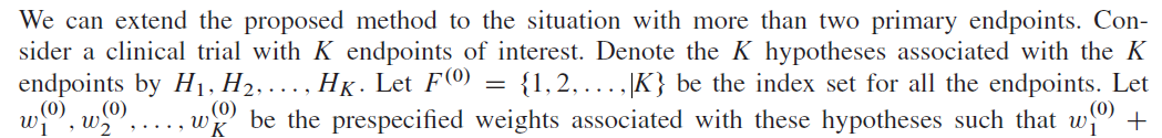
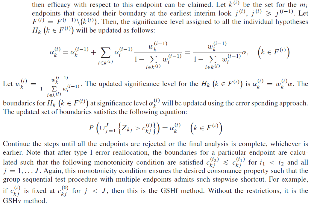
A proposed method to the situation with more than two primary endpoints.

Case 1 - MONET1
ClinicalTrials.gov Identifier: NCT00460317. Amgen discontinued the development of AMG706 because the trial did not meet its primary objective.
Yining et al. apply the group sequential Holm methods proposed in the above to an actual clinical trial. The MOtesanib Non-Small Cell Lung Cancer Efficacy and Tolerability (MONET1) study was a phase 3, placebo-controlled randomized oncology clinical trial.
The primary objectives of this study were to determine if motesanib in combination with chemotherapy would improve survival (两个人群的生存情况)
- in the overall study population and
- in subjects with adenocarcinoma histology (adenocarcinoma subpopulation).
The type I error (overall 0.025) was split between
the overall population (0.015, one-sided) and
the adenocarcinoma subpopulation (0.01, one-sided).
The study had 80% power requiring 742 deaths in the overall population to detect a hazard ratio of 1.25 and 80% power requiring 593 deaths in the adenocarcinoma subpopulation to detect a hazard ratio of 1.30. [基于事件数考虑生存终点,统计量为log-rank]
A total of 1060 subjects were enrolled including 70% with the adenocarcinoma histology.
An interim analysis was planned when 50% of the total deaths occurred in the overall population. The number of deaths for patients with adenocarcinoma histology was also close to the 50% target in the subpopulation at the interim analysis.
A negligible amount of type I error (0.00005, one-sided) was assigned at the interim for each hypothesis in the original design. [50%事件发生的情况下考虑做中期分析,中期分配的\(\alpha\)为0.00005]
To apply the GSHv method, we use the O’Brien–Fleming spending function as in following Equation.
$$ \alpha_{A,OF}(t_{1A})=2\Phi(-\frac{Z_{\alpha_{A}/2}}{\sqrt{t_{1A}}}), $$where \(\Phi(\cdot)\) is the standard normal cdf and \(Z_x\) is the \((1-x)\) quantile of the standard normal distribution.
The critical boundaries can be obtained by solving the following equations [注意是单侧显著性,其中\(X_1\)和\(X_2\)是logrank statistics at IA and Final Analysis for overall population]:

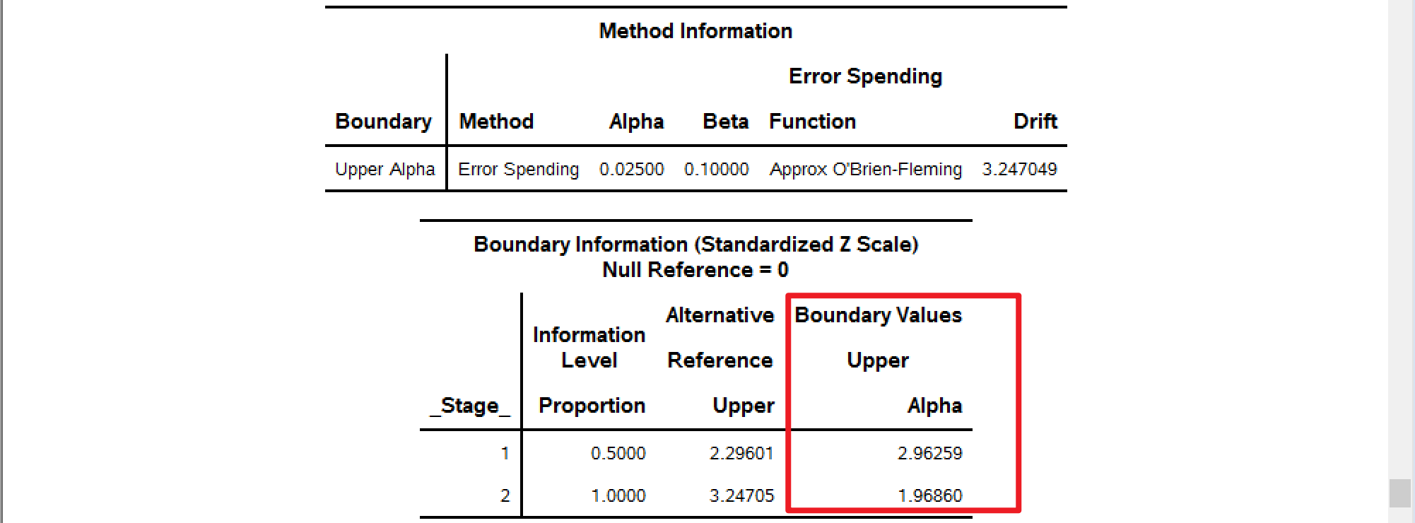
It can be shown that for the overall population
| \(c_1\) | \(c_1'\) | \(c_2\) | \(c_2'\) |
|---|---|---|---|
| 3.25 | 2.96 | 2.18 | 1.97 |
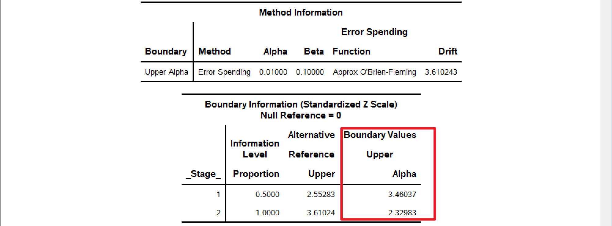
similarly, in the adenocarcinoma subpopulation
| \(d_1\) | \(d_1'\) | \(d_2\) | \(d_2'\) |
|---|---|---|---|
| 3.46 | 2.96 | 2.33 | 1.97 |
Similarly, if the GSHf is used with the same O’Brien–Fleming spending function, then critical boundaries can be obtained by solving

It can be shown that for the overall population
| \(c_1\) | \(c_2\) | \(c_2'\) |
|---|---|---|
| 3.25 | 2.18 | 1.96 |
similarly, in the adenocarcinoma subpopulation
| \(d_1\) | \(d_2\) | \(d_2'\) |
|---|---|---|
| 3.46 | 2.33 | 1.96 |
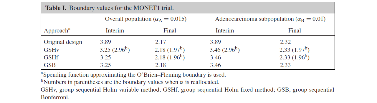
Table I summarizes the boundary values of the various methods.
In addition, Figures 1 and 2 illustrate the boundaries and the rejection regions of GSHf, GSHv, and GSB.
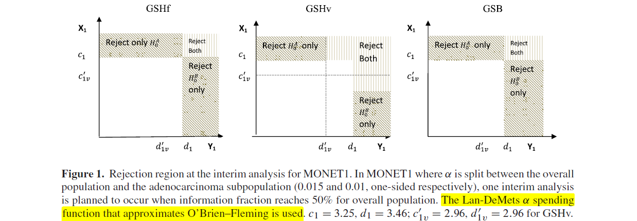
As shown in Figures 1 and 2C, the shaded areas representing rejection region for detecting significant effects for the overall population or subpopulation are identical for all methods.
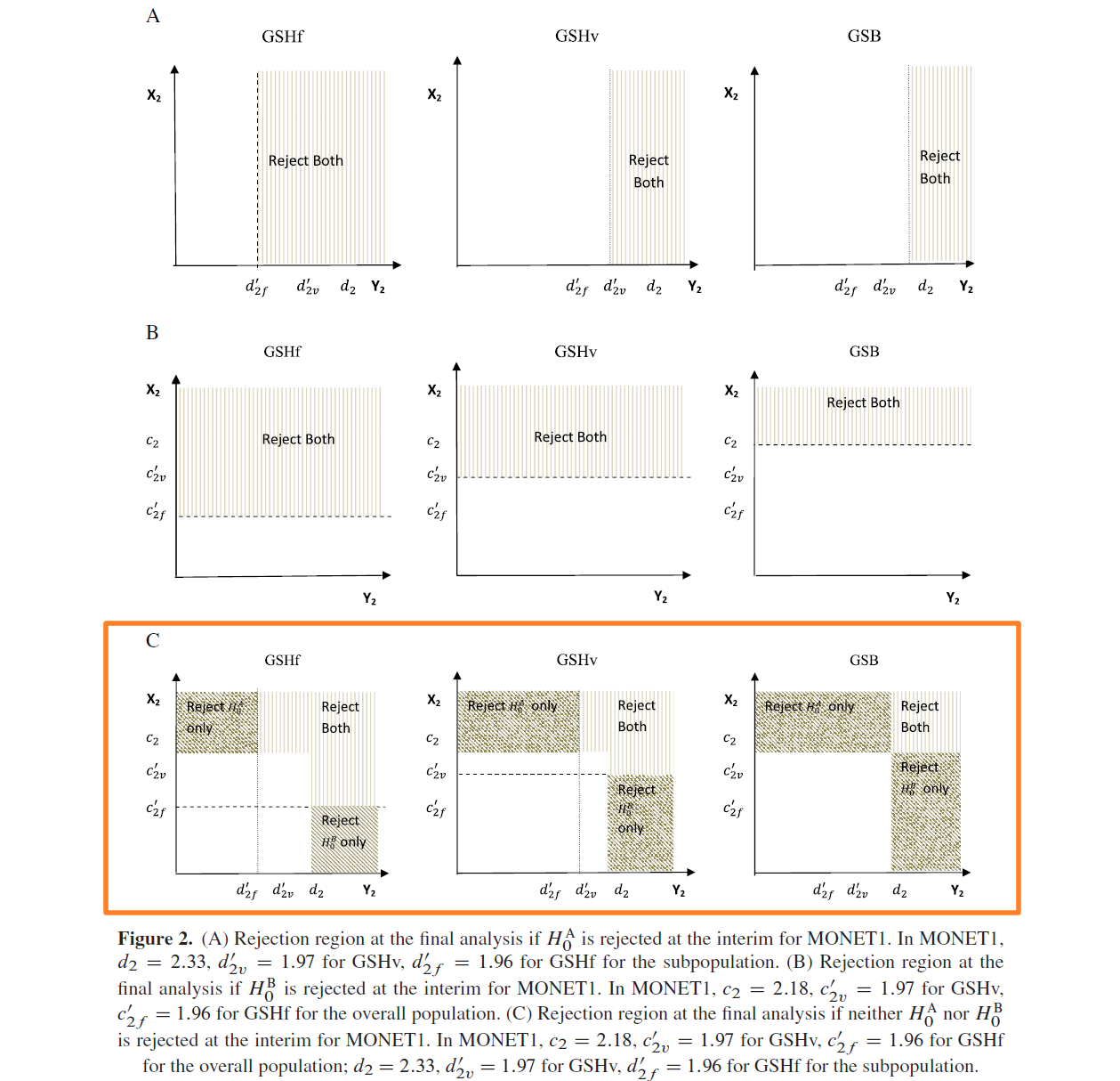
However, the rejection regions for detecting significant effects in both the overall and subpopulation are different, with the GSHf procedure having the largest area at the final analysis (Figure 2A–C) and the GSHv procedure having the largest area at the interim analysis (Figure 1).
The trial did not stop at the interim analysis. At the final analysis, the trial failed to demonstrate survival benefits of motesanib in either the overall population or the adenocarcinoma subpopulation.
参考文献:amgpaper.pdf
参考方案:amgprot.pdf
Discussion
本试验的主要终点为OS,人群为Overall Population和腺癌亚组人群,以下分别记为OS与OSAD。
生存终点OS和PFS使用的分析方法为Stratified log-rank test,HR的计算使用的方法为Cox Proportional hazards model。
OS与OSBM分得的\(\alpha\)分别为0.015与0.01(单侧);Overall population中发生50%死亡事件时执行期中分析,此时腺癌亚组人群的死亡事件占该人群的比例大概也是50%。期中分析分配给每个统计假设的一类错误水平为单侧0.00005。
O‘Brien-Fleming \(\alpha\)消耗函数为 \[ \alpha(t)=2-2\Phi(\frac{Z_{\alpha/2}}{\sqrt{t}})=2\Phi(-\frac{Z_{\alpha/2}}{\sqrt{t}}). \] ---
算法阐释
本试验有2个假设:\(H_{0A}\)和\(H_{0B}\) (数字代号 A:1,B:2);
令\(F^{(0)}=\left \{ 1,2 \right \}\)为假设的index set;
初始\(\alpha_A^{(0)}\)分配为0.015,对应权重为\(w_A^{(0)}=0.6\);终点B类似,初始\(\alpha_B^{(0)}\)分配为0.01, \(w_B^{(0)}=0.4\);
令\(Z_{A,j}\)为终点A在期中 \(j(j\le J)\) 时候的Wald统计量,终点B同理;
令\(c_{A,j}^{(0)}\)为终点A在期中 \(j(j\le J)\) 时候,对应\(\alpha_A^{(0)}\)的成组序贯边界(group sequential boundary, GSB),终点B同理。
以上条件下,成组序贯边界满足 (\(K\)为假设个数) \[ P[\bigcup_{j=1}^J(Z_{kj}>c_{kj})]=\alpha_k^{(0)},\text{ }k=1,2,\cdots,K \]
- 使用边界\(c_{A,j=1}^{(0)}\)与\(c_{B,j=1}^{(0)}\), 在\(\alpha_A^{(0)}\)与\(\alpha_B^{(0)}\)下检验假设\(H_{0A}\)和\(H_{0B}\)。 1.a. 若两个终点的Wald统计量都没跨越成组序贯边界,保留所有原假设,检验停止; 1.b. 若两个终点的Wald统计量\(Z_{A,j=1}\)或者\(Z_{B,j=1}\)中的一个,或者两个,在期中分析\(j^{(1)=1}\)的时间点时,跨越了成组序贯边界,那么可以宣告有效性。
- 假设这个场景中,在时间点\(j^{(1)=1}\)时,只有终点A的Wald统计量\(Z_{A,j=1}\)跨越了边界\(c_{A,j=1}^{(0)}\),那么此时可以宣布终点A的有效性,未检验通过的终点集合更新为。在这个时间点\(j^{(1)=1}\)时,还保留着的未拒绝的假设为\(H_{0B}\)。根据算法,此时终点\(H_{0B}\)的显著性水平权重需更新为 \[ \alpha_B^{(1)}=\frac{w_B^{(0)}}{1-w_A^{(0)}} \alpha=0.025\times \frac{0.4}{1-0.6}=0.025. \] 此时终点B的边界需要根据上述显著性水平,使用error spending function进行更新并且满足如下等式: \[ P[\bigcup_{j=1}^2(Z_{B,j}>c_{B,j}^{(1)})]=\alpha_B^{(1)}. \]
- 此时推进到Final analysis (\(j=J=2\))。此时的\(F^{(1)}=F^{(0)}\setminus \left \{ 1 \right \}=\left \{ 2 \right \}\)。假设此时的终点B的Wald检验统计量\(Z_{B,j=2}\)跨越了上述更新的\(c_{B,j=2}^{(1)}\),则宣告终点B的有效性,否则检验停止。
这样的步骤需要重复至所有的假设都被拒绝,或者完成最终分析。
SAS Code
主要演示边界值计算。选择SAS中的单侧error function去近似OF边界:OneSidedErrorSpending。1
2
3
4
5
6
7
8
9
10ods graphics on;
proc seqdesign plots=(errspend);
OneSidedErrorSpending: design nstages=2
method(alpha)=errfuncobf
alt=upper stop=REJECT
alpha=0.015
;
ods output Boundary=bd1;
run;
分别使用不同的alpha=去计算边界,alpha的取值可以为0.015,0.01,0.025 (full \(\alpha=0.025\))。
以下SAS计算结果可以与Table I中的GSBv进行对比。
alpha=0.015

alpha=0.01
alpha=0.025
Case 2 - HER2CLIMB (ONT-380-206)
Primary Objective
- To assess the effect of tucatinib vs. placebo in combination with capecitabine and trastuzumab on progression-free survival (PFS) per RECIST 1.1 based on blinded independent central review (BICR) [全人群]
Key Secondary Objectives
- To assess the effect of tucatinib vs. placebo in combination with capecitabine and trastuzumab on PFS in patients with a history of brain metastases or brain metastases at baseline or equivocal brain lesions at baseline using RECIST 1.1 based on BICR [亚组人群,脑转移,下文记为PFSBM]
- To assess the effects of tucatinib vs. placebo in combination with capecitabine and trastuzumab on overall survival (OS)
Sample Size
The sample size for this study was calculated based on maintaining 90% power for the primary endpoint PFS and 80% power for OS with an alpha level of 0.02.
For PFS, 288 events are required with 90% power to detect a hazard ratio of 0.67 (4.5 months median PFS in the control arm versus 6.75 months in the experimental arm) using a 2-sided log-rank test and alpha of 0.05.
For OS, 361 events are required with 80% power to detect a hazard ratio of 0.70 (15 months median OS in the control arm vs. 21.4 months in the experimental arm) using a 2-sided log-rank test and alpha of 0.02, taking into account of two interim analyses. With 361 OS events, it will provide 88% power using a 2-sided log-rank test with an alpha of 0.05.
For PFSBM, 220 events are required with 80% power to detect a hazard ratio of 0.67 (4.5 months median PFSBM in the control arm versus 6.75 months in the experimental arm) using a 2-sided log-rank test at alpha of 0.05, taking into account of one interim analysis. The power will be 74% at 2-sided alpha of 0.03.
Approximately 600 subjects will be randomized in a 2:1 ratio to either the experimental arm or the control arm. Assuming an accrual period of 48 months and a 5% yearly drop-out rate, it is expected that 361 OS events will be observed approximately 59 months after first subject randomized.
Sample size and power were calculated using EAST® version 6.4, by Cytel Inc.
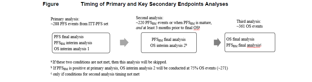
Timing of Analyses
The primary analysis of PFS will occur when approximately 288 PFS events determined by BICR have occurred in the ITT-PFS set and enrollment has been completed for the study. An interim analysis for the key secondary endpoints PFSBM and OS will also be performed at this time if PFS is statistically significant.
If PFSBM is statistically significant at the first interim analysis, no further formal testing of PFSBM will be conducted. The second interim analysis for OS will be performed when approximately 75% (271) of total OS events have occurred in the ITT-OS set, and the final OS analysis will be conducted after approximately 361 OS events have occurred in the ITT-OS set.
If PFSBM is not statistically significant at the first interim analysis, a second analysis of the key secondary endpoints will be performed when (a) approximately 220 PFSBM events have occured in the ITT-PFSBrainMets set or the PFSBM events are sufficiently mature (e.g. approximately less than 6 events are expected with 3 months additional follow up) and (b) at least 3 months before the projected OS final analysis. If both of the above conditions (a and b) are not met, this analysis of PFSBM and OS will not be conducted, and the OS final analysis at 361 OS events will also be the timing of the final PFSBM analysis.
No interim analyses for efficacy are planned for the primary endpoint.
One formal interim analysis for superiority is planned for the key secondary endpoint of PFSBM and two formal interim analyses for superiority are planned for the key secondary endpoint of OS if the primary analysis for PFS is statistically significant. The second interim analysis for OS may not be conducted as described above. The interim analyses will be conducted at the timing described above. The stopping boundaries will be determined using Lan-DeMets spending functions for the O'Brien and Fleming boundaries. See next section for control of multiplicity.
The timing of analyses for the primary and key secondary endpoints are illustrated in Figure
Multiple Comparison/Multiplicity
To maintain strong control of the family-wise type I error rate at 0.05, the PFS will be tested at 0.05 level first in the ITT-PFS set, if it is significant, then the key secondary endpoints will be tested using the group sequential Holm variable (GSHv) procedure.
The \(\alpha\) split between PFSBM and OS is \(\alpha=0.03\) and \(\alpha=0.02\), respectively, and each one will be tested at the interim analysis(s) and again at the final analysis, if not rejected at the interim analysis. The information fraction t is the ratio between number of events at interim analysis and number of events at final analysis. For illustration purpose, we assume \(t=0.812\) for PFSBM and \(t_1=0.626\), \(t_2=0.779\) for the two interim analyses for OS.
The boundary at interim analysis is determined according to the Lan-DeMets O’Brien-Fleming (LD(OF)) approximation spending function LD(OF): \(\alpha(t)=4-4\Phi(\frac{Z_{\alpha/4}}{\sqrt{t}})\) for 2-sided tests, where \(\alpha/4\) is the upper \(\alpha/4\) critical point of the standard normal distribution.
The GSHv procedure operates as follows.
- Begin with a 0.03-level group sequential boundary for PFSBM and a 0.02-level group sequential boundary for OS. The corresponding boundaries for the two endpoints are given in Table 1. If both of the endpoints are found significant at analysis 1 (primary analysis), then no more formal statistical testing for PFSBM and OS will be conducted.


- If only one endpoint is found significant at the analysis 1 (primary analysis) then the \(\alpha\) can be recycled to the other endpoint: If PFSBM is significant at interim but OS is not then the \(\alpha\) will be recycled from PFSBM to OS and use a 0.05-level LD(OF) boundary for OS. On the other hand, if OS is significant at analysis 1 (primary analysis) but PFSBM is not then the \(\alpha\) will be recycled from OS to PFSBM and use a 0.05-level LD(OF) boundary for PFSBM. The corresponding 0.05-level LD(OF) boundaries are given in Table 2. The unrejected hypothesis can be re-tested at the current and future analysis using the modified boundaries.
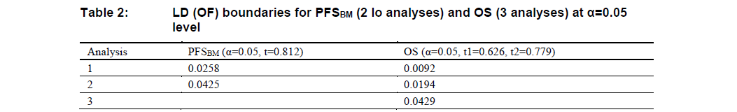
If neither of the endpoints is found significant at analysis 1 (primary analysis), then both endpoints will be tested again at analysis 2. The initial boundaries for final analysis follow Table 1 (analysis 2). If only one endpoint is found significant by these initial boundaries, then the other one can be tested again using the modified boundary as shown in Table 2 (analysis 2). For example, if PFSBM was found significant at final analysis at \(\alpha=0.0259\) level, but OS was not significant at \(\alpha=0.0069\) level, then OS can be tested again at the \(\alpha=0.0194\) level.
If PFSBM is significant at analysis 1 or 2, the boundary of OS analysis at analysis 3 is 0.0429; otherwise, the boundary for OS analysis at analysis 3 is 0.0176.
Note that the boundaries presented in the tables will be adjusted with the actual information fraction.
As detailed in the timing of analysis part, the second interim analysis for OS may not be conducted, which means both PFSBM and OS will have at most 2 analyses. In that case, LD(OF) boundaries at each analysis will be modified as illustrated in Table 3 and Table 4.


Similar to Table 1 and Table 2, the information fraction (\(t\)) in Table 3 and Table 4 are for illustration purpose only.
If both PFSBM and OS are statistically significant, the secondary endpoint of ORR by BICR in the ITT-OS set will be formally tested between two treatment arms at the two sided \(\alpha=0.05\) level.
Appendix - Lan-DeMets Spending function overview
Lan and DeMets (1983) first published the method of using spending functions to set boundaries for group sequential trials.
In this publication they proposed two specific spending functions: one to approximate an O'Brien-Fleming design and the other to approximate a Pocock design. The spending function to approximate O'Brien-Fleming has been generalized as proposed by Liu, et al (2012)
The Lan-DeMets (1983) spending function to approximate an O'Brien-Fleming bound is implemented in the function:
\[ f(t; \alpha)=2-2\Phi\left(\Phi^{-1}(1-\alpha/2)/ t^{\rho/2}\right). \]
The Lan-DeMets (1983) spending function to approximate a Pocock design is implemented in the function:
\[ f(t;\alpha)=\alpha ln(1+(e-1)t). \]
Reference
Ye, Y., Li, A., Liu, L., & Yao, B. (2013). A group sequential Holm procedure with multiple primary endpoints. Statistics in medicine, 32(7), 1112–1124. https://doi.org/10.1002/sim.5700
Kantoff PW, Higano CS, Shore ND, Berger ER, Small EJ, Penson DF, Redfern CH, Ferrari AC, Dreicer R, Sims RB, Xu Y, Frohlich MW, Schellhammer PF. Sipuleucel-T immunotherapy for castration-resistant prostate cancer. The New England Journal of Medicine 2010; 363:411–422.
Bretz F, Maurer W, Brannath W, Posch M. A graphical approach to sequentially rejective multiple test procedures. Statistics in Medicine 2009; 28:586–604.
Lan, KKG and DeMets, DL (1983), Discrete sequential boundaries for clinical trials. Biometrika;70: 659-663.
Liu, Q, Lim, P, Nuamah, I, and Li, Y (2012), On adaptive error spending approach for group sequential trials with random information levels. Journal of biopharmaceutical statistics; 22(4), 687-699.