Background

This paper recommends using the UN structure with a new approach to analyze longitudinal data from randomized clinical trials. The approach proposed in this paper can assist in the convergence when the UN structure is used.

The paper investigates the following issues:

• biases in the regression parameter estimates as the result of misspecification of the covariance structure;
• comparison of the model-based and sandwich variance estimators;
• approaches to the convergence problem with UN covariance.

A Review of Approaches for Convergence Problems

The following reasons may lead to the convergence problem when using PROC MIXED with UN structure in SAS (using the default Newton-Raphson algorithm):

• an excessive amount of missing data,
• high correlations among repeated measures,
• a large number of time points.

Two common methods could be tried for resolving the convergence issues:

1. use the Fisher scoring algorithm (SCORING option of the PROC MIXED statement) to obtain the initial values of the covariance parameters;
2. use the no-diagonal factor analytic structure (via TYPE=FA0(T) option of the REPEATED statement, where T is the total number of time points), which effectively performs the Cholesky decomposition of the covariance matrix and is numerically more stable.

This paper also proposes a new method referred to as the Successive Univariate Regression Method.

Successive Univariate Regression Method

Suppose there are a total of \(T\) time points where the measurements of a continuous response is to be collected.

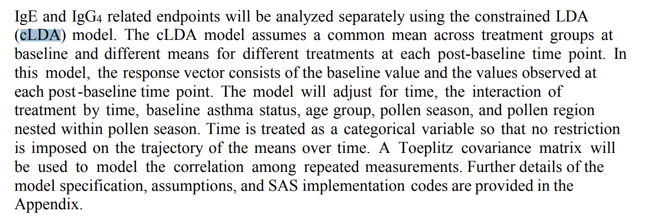
A Constrained Longitudinal Data Analysis (cLDA) model will be used for the analysis.

cLDA Model

An example description of cLDA model is shown in the following screenshot from a SAP:

(source: https://classic.clinicaltrials.gov/ProvidedDocs/98/NCT02478398/SAP_001.pdf)

Algorithm

Let \(A\) denote the treatment group;

Let \(X\) denote the other baseline variables.

The model for the full data collected on a subject is:

Step 1

Fit a series of univariate regression models.

Fit \(\left \{y_1 \mid X \right \}\), and then fit \(\left \{y_t \mid y_1, y_2, \cdots, y_{t-1},A,X \right \}\) successively for \(t=2,3,\cdots,T\).

We also use the notations for covariance parameters as follows:

• the resulting variance estimate in the regression model \(\left \{y_1 \mid X \right \}\): \(\hat{\sigma}_{11}\).
• the variance estimate in \(\left \{y_t \mid y_1, y_2, \cdots, y_{t-1},A,X \right \}\): \(\hat{\sigma}_{tt \cdot 1...t-1}\)
• the estimated coefficient associated with \(y_s\) in \(\left \{y_t \mid y_1, y_2, \cdots, y_{t-1},A,X \right \}\) for \(1 \le s \lt t \le T\): \(\hat{\phi}_{ts}\).

The notation of "\(\hat{\sigma}_{tt \cdot 1...t-1}\)" means that the estimated variance \(\hat{\sigma}_{tt}\) is obtained conditional on time points \(t-1\) to \(1\).

Step 2

Construct the covariance parameters: \(\left \{\sigma_{st}:1\le s,t\le T \right \}\) from parameters in the univariate regression models. By (1),

Consequently, we can successively apply the following matrix operations to obtain an initial estimate of the covariance parameters,

for \(t=2,3,\cdots T\).

Note that : \(\hat{\sigma}_{tt \cdot 1...t-1}\) is NOT THE SAME as \(\hat{\sigma}_{tt}\). The \(\hat{\sigma}_{tt \cdot 1...t-1}\) is obtained from the univariate regression from the Step 1, but the latter \(\hat{\sigma}_{tt}\) will be the initial guess for PARMS Statement in SAS.

For example, \(\hat{\sigma}_{T-1,T-1 \cdot 1...T-2}\)=\(\hat{\sigma}_{T-1,T-1}+\sum_{T-2}^{s=1}\hat{\phi}_{T-1,s}\hat{\sigma}_{T-1,s}\) for \(t=T-1\).

The (2) can be rewritten as \[ \hat{\sigma}_{ts}=\sum_{k=1}^{t-1}{\hat{\phi}_{tk}\hat{\sigma}_{sk}} \] for \(s=1,2,3,\cdots,t-1\), where \(\hat{\sigma}_{sk}=\hat{\sigma}_{ks}\) for \(k=s+1,\cdots,t-1\).

Consequently, no matrix inversion is needed for constructing the covariance parameters.

Once an initial estimate of the covariance matrix is obtained, it can be used in the PARMS statement in PROC MIXED to start the iterative algorithm.

Discussion

If the default Newton–Raphson algorithm used by SAS PROC MIXED fails to converge, the Fisher scoring algorithm, the factor analytic structure, and the proposed successive univariate regression method can be tried in turn.

This usually resolves most convergence issues.

In the rare case where the above strategy fails, it is prudent to examine the data configuration and the model specification. If no data or model issues are identified, progressively more specific covariance structures (e.g. Toeplitz → AR(1)+random effect) may be tried to minimize the impact of misspecification, and we recommend the sandwich variance estimator to be used with structured covariance models to control the Type I error for large samples.

Reference

Lu, K., & Mehrotra, D. V. (2010). Specification of covariance structure in longitudinal data analysis for randomized clinical trials. Statistics in medicine, 29(4), 474–488. https://doi.org/10.1002/sim.3820

Download Link: https://www.stat.ubc.ca/~rollin/papers/LuCovarianceSIM2009.pdf